---
title: "S1. Chlorophyll-a bloom detection"
subtitle: "Mapping the study area and estimating seasonal bloom onset"
unnumbered: true
toc: true
toc-depth: 3
---
::: lead
This chapter describes how chlorophyll-a bloom onset was estimated from satellite-derived time series. We first provide geographic context for Isla Isabel and the chlorophyll extraction area, then describe the bloom detection algorithm, compare seasonal-window definitions, and visualize the resulting onset-date distributions.
:::
```{r}
#| label: setup-bloom-onset
#| include: false
# For data manipulation and plotting (loads ggplot2, dplyr, tidyr, etc.)
library(tidyverse)
# For handling and plotting spatial data
library(sf)
library(rnaturalearth)
library(ggspatial)
# For combining plots
library(cowplot) # Used for the map insets
library(patchwork) # Used for the final density plots
# For file path management
library(here)
# For time-series calculations (rolling medians)
library(zoo)
# For creating interactive HTML tables
library(DT)
```
## S1.1 Study area
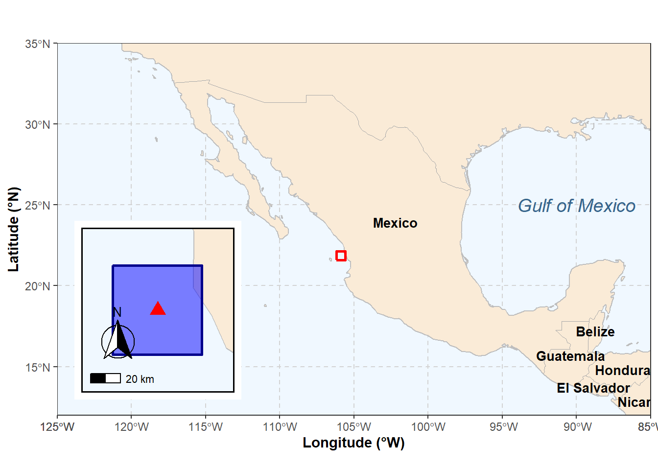
The figure below provides geographic context for Isla Isabel, Mexico, showing the island’s location in the eastern tropical Pacific and the focal extraction polygon used to obtain chlorophyll-a data for bloom detection.
```{r}
#| label: fig-isla-isabel-map
#| fig-width: 10
#| fig-height: 8
#| fig-cap: "Location of Isla Isabel, Mexico, and the focal extraction polygon used to derive chlorophyll-a time series. The main panel shows the broader eastern tropical Pacific and adjacent landmass, whereas the inset shows Isla Isabel and the extraction area in detail."
#| code-fold: true
#| code-summary: "Show code"
# --- Define Data ---
# Define the polygon coordinates
latitudes <- c(22.1203, 22.1203, 21.5797, 21.5797, 22.1203)
longitudes <- c(-106.1763, -105.5937, -105.5937, -106.1763, -106.1763)
coords_df <- data.frame(lon = longitudes, lat = latitudes)
polygon_sf <- st_polygon(list(as.matrix(coords_df)))
polygon_sf <- st_sfc(polygon_sf, crs = 4326)

# Define the marker coordinates for Isla Isabel
marker_lat_deg <- 21 + 50/60 + 59.0/3600
marker_lon_deg <- -(105 + 52/60 + 54.0/3600)
marker_point_df <- data.frame(lon = marker_lon_deg, lat = marker_lat_deg)
marker_point_sf <- st_point(c(marker_point_df$lon, marker_point_df$lat))
marker_point_sf <- st_sfc(marker_point_sf, crs = 4326)

# Get world map data
world <- ne_countries(scale = "medium", returnclass = "sf")
coastlines <- ne_coastline(scale = "medium", returnclass = "sf")

# Create points for country labels
world_points <- cbind(world, st_coordinates(st_centroid(world$geometry)))

# --- Main Map (Zoomed Out - Pacific Coast) ---
main_map <- ggplot() +
  # TYPO FIX: Changed "antiquhite" to "antiquewhite"
  geom_sf(data = world, fill = "antiquewhite", color = "darkgray") +
  geom_sf(data = coastlines, color = "grey", size = 0.5) +
  geom_sf(data = st_as_sfc(st_bbox(polygon_sf)), fill = NA, color = "red", size = 1) +
  geom_text(data = world_points, aes(x = X, y = Y, label = name),
            color = "black", size = 3.5, fontface = "bold", check_overlap = TRUE) +
  annotate(geom = "text", x = -90, y = 25, label = "Gulf of Mexico",
           fontface = "italic", color = "steelblue4", size = 5) +
  coord_sf(xlim = c(-125, -85), ylim = c(12, 35), expand = FALSE) +
  labs(title = "", x = "Longitude (°W)", y = "Latitude (°N)") +
  theme_bw() +
  theme(
    plot.title = element_text(hjust = 0.5, face = "bold"),
    axis.title = element_text(face = "bold"),
    panel.grid.major = element_line(color = "lightgray", linetype = "dashed"),
    panel.background = element_rect(fill = "aliceblue")
  )

# --- Inset Map (Zoomed In on Isla Isabel) ---
inset_map <- ggplot() +
  geom_sf(data = world, fill = "antiquewhite", color = "darkgray") +
  geom_sf(data = coastlines, color = "grey", size = 0.5) +
  geom_sf(data = polygon_sf, fill = "blue", alpha = 0.5, color = "darkblue", size = 1) +
  geom_sf(data = marker_point_sf, color = "red", size = 4, shape = 17) +
  geom_text(data = marker_point_df, aes(x = lon, y = lat), label = "Isla Isabel", hjust = 0.5, vjust = -5.5, color = "black", fontface = "bold", size = 6) +
  annotation_scale(location = "bl", width_hint = 0.2) +
  annotation_north_arrow(
    location = "bl", which_north = "true",
    pad_x = unit(0.09, "in"), pad_y = unit(0.3, "in"),
    style = north_arrow_fancy_orienteering
  ) +
  coord_sf(
    xlim = c(marker_lon_deg - 0.5, marker_lon_deg + 0.5),
    ylim = c(marker_lat_deg - 0.5, marker_lat_deg + 0.5),
    expand = FALSE
  ) +
  theme_bw() +
  theme(
    axis.text = element_blank(),
    axis.ticks = element_blank(),
    axis.title = element_blank(),
    panel.grid.major = element_blank(),
    panel.grid.minor = element_blank(),
    panel.background = element_rect(fill = "aliceblue"),
    panel.border = element_rect(color = "black", fill = NA, linewidth = 1)
  )

# --- Combine Maps using cowplot ---
mapIS<-ggdraw() +
  draw_plot(main_map) +
  draw_plot(inset_map, x = 0.05, y = 0.15, width = 0.38, height = 0.38)
```
```{r}
#| echo: false
mapIS
```
```{r}
#| label: save_map
#| eval: false
ggsave(filename = here("..","Plots", "Map_Isla_Isabel.pdf"),
       plot = mapIS,
       dpi = 300, device = cairo_pdf)

ggsave(filename = here("..","Plots", "Map_Isla_Isabel.jpg"),
       plot = mapIS,
       width = 7,
       height = 7,
       dpi = 300)
```
## S1.2 Bloom onset estimation
This section describes the procedure used to estimate phytoplankton bloom onset from satellite-derived chlorophyll-a time series. We used dynamic, season-specific thresholds based on the median chlorophyll-a concentration within each seasonal window, and identified bloom onset as the first sustained increase above threshold.
::: {.callout-note appearance="simple"}
## Detection logic
For each seasonal window, bloom onset was defined as the first day on which chlorophyll-a exceeded a season-specific threshold for two consecutive 7-day rolling medians. This criterion was used to identify sustained increases rather than short-lived spikes.
:::
### Workflow
The bloom detection workflow consisted of three steps: loading and cleaning the chlorophyll-a time series, estimating bloom onset under two alternative seasonal-window definitions, and summarizing the resulting onset dates across thresholds.
## Load chlorophyll-a data.
```{r}
#| label: chlorophyll data
CHL_df <- read.csv(here("..","data", "MODIS.CHL.R2022.csv"), header = TRUE) %>%
  drop_na() %>%
  dplyr::select(date, chlorophyll) %>%
  rename(daily_value = chlorophyll)

CHL_df <- CHL_df %>%
  mutate(date = dmy(date))
```
## Estimate sustained bloom onset
The same detection logic was applied under both seasonal-window definitions:
- **Seasonal window:** either Winter–Spring (21 December–20 June) or Autumn–Spring (21 September–20 June)
- **Baseline:** the median chlorophyll-a concentration within each seasonal window
- **Thresholds:** 5%, 15%, 25%, and 30% above the seasonal median
- **Sustained increase criterion:** the first day for which two consecutive 7-day rolling medians exceeded the threshold
- **Output:** bloom onset date, chlorophyll-a value at onset, and the threshold value for that season
::: panel-tabset
## Winter–Spring window
This version defines the seasonal window from 21 December of the previous year to 20 June of the focal year.
```{r}
#| label: bloom-function-winter-spring
#| code-fold: true
#| code-summary: "Show code"
calculate_sustained_bloom_start <- function(data_frame, value_column_name = "daily_value", min_duration_days = 7) {

  thresholds <- c(0.05, 0.15,0.25, 0.30)

  # Prepare and annotate data
  data_frame <- data_frame %>%
    mutate(date = as.Date(date)) %>%
    arrange(date) %>%
    mutate(season_year = ifelse(month(date) == 12, year(date) + 1, year(date)))

  # Define seasonal window
  season_ranges <- data_frame %>%
    distinct(season_year) %>%
    mutate(
      season_start_date = ymd(paste0(season_year - 1, "-12-21")),
      season_end_date = ymd(paste0(season_year, "-06-20"))
    )

  # Filter seasonal data
  seasonal_data <- data_frame %>%
    left_join(season_ranges, by = "season_year") %>%
    filter(date >= season_start_date & date <= season_end_date) %>%
    arrange(season_year, date)

  # Compute yearly medians
  medians <- seasonal_data %>%
    group_by(season_year) %>%
    summarise(yearly_median = median(!!sym(value_column_name), na.rm = TRUE), .groups = "drop")

  # Initialize final result with medians
  all_results <- medians
  bloom_date_raws <- list()

  for (thr in thresholds) {
    label <- paste0("thr", thr * 100)

    # Add threshold column
    threshold_tbl <- medians %>%
      mutate(threshold = yearly_median * (1 + thr))

    seasonal_thr_data <- seasonal_data %>%
      left_join(threshold_tbl, by = "season_year")

    # Compute rolling medians
    seasonal_thr_data <- seasonal_thr_data %>%
      group_by(season_year) %>%
      mutate(
        rolling_median_week1 = rollapply(
          !!sym(value_column_name), min_duration_days, median, na.rm = TRUE, fill = NA, align = "left"
        ),
        rolling_median_week2 = rollapply(
          lead(!!sym(value_column_name), n = min_duration_days), min_duration_days, median, na.rm = TRUE, fill = NA, align = "left"
        ),
        cond_i = !is.na(rolling_median_week1) & rolling_median_week1 >= threshold,
        cond_ii = !is.na(rolling_median_week2) & rolling_median_week2 >= threshold
      ) %>%
      filter(cond_i & cond_ii) %>%
      summarise(bloom_date = min(date, na.rm = TRUE), .groups = "drop")

    # Store raw date for difference calculation
    bloom_date_raws[[label]] <- seasonal_thr_data %>%
      rename(!!paste0("bloom_date_raw_", label) := bloom_date)

    # Join back to get bloom values and threshold
    enriched <- seasonal_thr_data %>%
      left_join(seasonal_data, by = "season_year") %>%
      group_by(season_year) %>%
      summarise(
        !!paste0("bloom_start_", label) := format(first(bloom_date), "%d/%m/%Y"),
        !!paste0("value_at_bloom_", label) := seasonal_data[[value_column_name]][match(first(bloom_date), seasonal_data$date)],
        !!paste0("threshold_", label) := medians$yearly_median[medians$season_year == first(season_year)] * (1 + thr),
        .groups = "drop"
      )

    # Join enriched info to results
    all_results <- all_results %>%
      left_join(enriched, by = "season_year")
  }

  # Join all bloom date raws
  bloom_date_df <- reduce(bloom_date_raws, left_join, by = "season_year")

  # Add differences between 5% vs 15% and 30%
  all_results <- all_results %>%
    left_join(bloom_date_df, by = "season_year") %>%
    mutate(
      diff_days_5_vs_15 = as.numeric(bloom_date_raw_thr15 - bloom_date_raw_thr5),
      diff_days_5_vs_30 = as.numeric(bloom_date_raw_thr30 - bloom_date_raw_thr5)
    ) %>%
    select(-starts_with("bloom_date_raw_"))

  return(all_results)
}
 bloom_startsA <- calculate_sustained_bloom_start(CHL_df)
#write.csv(bloom_starts2, here("data", "bloom_dates.csv"), row.names = FALSE)
```
## Autumn–Spring window
This version defines the seasonal window from 21 September of the previous year to 20 June of the focal year.
```{r}
#| label: bloom-function-autumn-spring
#| code-fold: true
#| code-summary: "Show code"
calculate_sustained_bloom_startB <- function(data_frame, value_column_name = "daily_value", min_duration_days = 7) {

  thresholds <- c(0.05, 0.15,0.25, 0.30)

  # Prepare and annotate data
  data_frame <- data_frame %>%
    mutate(date = as.Date(date)) %>%
    arrange(date) %>%
    mutate(season_year = ifelse(month(date) == 9, year(date) + 1, year(date)))

  # Define seasonal window
  season_ranges <- data_frame %>%
    distinct(season_year) %>%
    mutate(
      season_start_date = ymd(paste0(season_year - 1, "-09-21")),
      season_end_date = ymd(paste0(season_year, "-06-20"))
    )

  # Filter seasonal data
  seasonal_data <- data_frame %>%
    left_join(season_ranges, by = "season_year") %>%
    filter(date >= season_start_date & date <= season_end_date) %>%
    arrange(season_year, date)

  # Compute yearly medians
  medians <- seasonal_data %>%
    group_by(season_year) %>%
    summarise(yearly_median = median(!!sym(value_column_name), na.rm = TRUE), .groups = "drop")

  # Initialize final result with medians
  all_results <- medians
  bloom_date_raws <- list()

  for (thr in thresholds) {
    label <- paste0("thr", thr * 100)

    # Add threshold column
    threshold_tbl <- medians %>%
      mutate(threshold = yearly_median * (1 + thr))

    seasonal_thr_data <- seasonal_data %>%
      left_join(threshold_tbl, by = "season_year")

    # Compute rolling medians
    seasonal_thr_data <- seasonal_thr_data %>%
      group_by(season_year) %>%
      mutate(
        rolling_median_week1 = rollapply(
          !!sym(value_column_name), min_duration_days, median, na.rm = TRUE, fill = NA, align = "left"
        ),
        rolling_median_week2 = rollapply(
          lead(!!sym(value_column_name), n = min_duration_days), min_duration_days, median, na.rm = TRUE, fill = NA, align = "left"
        ),
        cond_i = !is.na(rolling_median_week1) & rolling_median_week1 >= threshold,
        cond_ii = !is.na(rolling_median_week2) & rolling_median_week2 >= threshold
      ) %>%
      filter(cond_i & cond_ii) %>%
      summarise(bloom_date = min(date, na.rm = TRUE), .groups = "drop")

    # Store raw date for difference calculation
    bloom_date_raws[[label]] <- seasonal_thr_data %>%
      rename(!!paste0("bloom_date_raw_", label) := bloom_date)

    # Join back to get bloom values and threshold
    enriched <- seasonal_thr_data %>%
      left_join(seasonal_data, by = "season_year") %>%
      group_by(season_year) %>%
      summarise(
        !!paste0("bloom_start_", label) := format(first(bloom_date), "%d/%m/%Y"),
        !!paste0("value_at_bloom_", label) := seasonal_data[[value_column_name]][match(first(bloom_date), seasonal_data$date)],
        !!paste0("threshold_", label) := medians$yearly_median[medians$season_year == first(season_year)] * (1 + thr),
        .groups = "drop"
      )

    # Join enriched info to results
    all_results <- all_results %>%
      left_join(enriched, by = "season_year")
  }

  # Join all bloom date raws
  bloom_date_df <- reduce(bloom_date_raws, left_join, by = "season_year")

  # Add differences between 5% vs 15% and 30%
  all_results <- all_results %>%
    left_join(bloom_date_df, by = "season_year") %>%
    mutate(
      diff_days_5_vs_15 = as.numeric(bloom_date_raw_thr15 - bloom_date_raw_thr5),
      diff_days_5_vs_30 = as.numeric(bloom_date_raw_thr30 - bloom_date_raw_thr5)
    ) %>%
    select(-starts_with("bloom_date_raw_"))

  return(all_results)
}
bloom_startsB <- calculate_sustained_bloom_startB(CHL_df)
#write.csv(bloom_startsB, here("data", "bloom_datesB.csv"), row.names = FALSE)
```
:::
### Summary tables
The tables below summarize estimated bloom onset dates under the two seasonal-window definitions. These outputs were used to compare the robustness of onset estimates across threshold choices and seasonal boundaries.
::: panel-tabset
## Winter–Spring results
This table summarizes estimated bloom onset dates for the Winter–Spring seasonal window (21 December–20 June).
```{r}
#| label: Summary A
#| echo: false
DT::datatable(
bloom_startsA,
options = list(
pageLength = 10,
scrollX = TRUE,
dom = 'Bfrtip',
buttons = c('copy', 'csv')
),
extensions = 'Buttons',
rownames = FALSE
) %>%
formatRound(columns = c("yearly_median","value_at_bloom_thr5", "threshold_thr5","value_at_bloom_thr15","threshold_thr15","value_at_bloom_thr25","threshold_thr25","value_at_bloom_thr30","threshold_thr30"), digits = 3)%>%
formatStyle(columns = names(bloom_startsA), `text-align` = 'center')
```
## Autumn–Spring results
This table summarizes estimated bloom onset dates for the Autumn–Spring seasonal window (21 September–20 June).
```{r}
#| label: Summary B
#| echo: false
DT::datatable(
bloom_startsB,
options = list(
pageLength = 10,
scrollX = TRUE,
dom = 'Bfrtip',
buttons = c('copy', 'csv')
),
extensions = 'Buttons',
rownames = FALSE
) %>%
formatRound(columns = c("yearly_median","value_at_bloom_thr5", "threshold_thr5","value_at_bloom_thr15","threshold_thr15","value_at_bloom_thr25","threshold_thr25","value_at_bloom_thr30","threshold_thr30"), digits = 3)%>%
formatStyle(columns = names(bloom_startsB), `text-align` = 'center')
```
:::
## S1.3 Visualization of chlorophyll-a bloom onset dates
To compare bloom timing across years, thresholds, and seasonal-window definitions, bloom onset dates were transformed to a common seasonal calendar and plotted as distributions.
### Data processing for visualization
Before plotting, bloom onset estimates were reshaped to long format and standardized to a common seasonal calendar. Dates falling in September–December were assigned to year 2000, whereas dates falling in January–June were assigned to year 2001. This made it possible to compare timing distributions across thresholds and seasonal windows independently of calendar year.
```{r}
#| label: Frequency of bloom start dates
#| code-fold: true
#| code-summary: "Show code"
process_for_plotting <- function(results) {
  results %>%
    select(season_year, starts_with("bloom_start_")) %>%
    pivot_longer(
      cols = -season_year,
      names_to = "threshold_id",
      values_to = "bloom_date_str",
      values_drop_na = TRUE
    ) %>%
    mutate(
      threshold_label = gsub("bloom_start_thr", "", threshold_id),
      threshold = factor(paste0(threshold_label, "%"), levels = c("5%", "15%", "25%", "30%")),
      bloom_date = dmy(bloom_date_str),
      bloom_day_month = if_else(
          month(bloom_date) >= 9,
          update(bloom_date, year = 2000),
          update(bloom_date, year = 2001)
      )
    )
}

bloom_dates_long_A <- process_for_plotting(bloom_startsA)
bloom_dates_long_B <- process_for_plotting(bloom_startsB)


sample_sizes_A <- bloom_dates_long_A %>%
  group_by(threshold) %>%
  summarise(label = paste("n =", n_distinct(season_year)), .groups = "drop")

sample_sizes_B <- bloom_dates_long_B %>%
  group_by(threshold) %>%
  summarise(label = paste("n =", n_distinct(season_year)), .groups = "drop")


mean_dates_A <- bloom_dates_long_A %>%
  group_by(threshold) %>%
  summarise(mean_date = as.Date(mean(as.numeric(bloom_day_month)), origin = "1970-01-01"), .groups = "drop")

mean_dates_B <- bloom_dates_long_B %>%
  group_by(threshold) %>%
  summarise(mean_date = as.Date(mean(as.numeric(bloom_day_month)), origin = "1970-01-01"), .groups = "drop")
```
### Generating and combining onset-date distribution plots
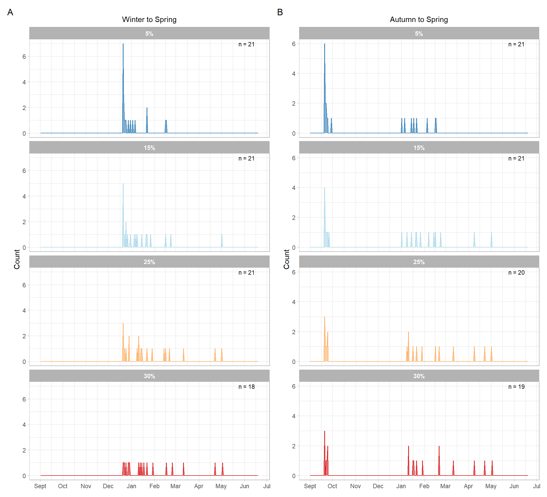
Binned area plots were generated for each seasonal window and faceted by threshold level. Panel labels indicate the number of seasons with a detected bloom onset for each threshold. The Winter–Spring and Autumn–Spring panels were combined for side-by-side comparison.
```{r}
#| label: Area plot of bloom start dates
#| code-fold: true
#| code-summary: "Show code"
# --- Define the color palette once ---
bloom_colors <- c("5%"="#2c7bb6", "15%"="#abd9e9", "25%"="#fdae61", "30%"="#d7191c")

# --- Plot A ---
area_plot_A <- ggplot(bloom_dates_long_A,
                      # Add 'color' aesthetic
                      aes(x = bloom_day_month, fill = threshold, color = threshold)) +


  geom_area(
    stat = "bin",
    binwidth = 1,
    boundary = 0,
    alpha = 0.6,          # Adjusted alpha for better overlap
    position = "identity",
    linewidth = 0.5       # Controls outline thickness
  ) +

  geom_text(data = sample_sizes_A, aes(x = as.Date("2001-06-15"), y = Inf, label = label), vjust = 1.5, hjust = 1, size = 3, inherit.aes = FALSE) +
  facet_wrap(~threshold, ncol = 1, scales = "fixed") +
  labs(subtitle = "Winter to Spring", x = NULL, y = "Count") +
  theme_light() +
  scale_fill_manual(values = bloom_colors) +
  scale_color_manual(values = bloom_colors) +
  scale_x_date(limits = c(as.Date("2000-09-01"), as.Date("2001-06-20")), date_labels = "%b", date_breaks = "1 month") +
  theme(plot.subtitle = element_text(hjust = 0.5), legend.position = "none", strip.text = element_text(face = "bold"))

# --- Plot B ---
area_plot_B <- ggplot(bloom_dates_long_B,

                      aes(x = bloom_day_month, fill = threshold, color = threshold)) +


  geom_area(
    stat = "bin",
    binwidth = 1,
    boundary = 0,
    alpha = 0.6,
    position = "identity",
    linewidth = 0.5
  ) +

  facet_wrap(~threshold, ncol = 1, scales = "fixed") +
  geom_text(data = sample_sizes_B, aes(x = as.Date("2001-06-15"), y = Inf, label = label), vjust = 1.5, hjust = 1, size = 3, inherit.aes = FALSE)+
  labs(subtitle = "Autumn to Spring", x = NULL, y = "Count") +
  theme_light() +
  scale_fill_manual(values = bloom_colors) +
  scale_color_manual(values = bloom_colors) +
  scale_x_date(limits = c(as.Date("2000-09-01"), as.Date("2001-06-20")), date_labels = "%b", date_breaks = "1 month") +
  theme(plot.subtitle = element_text(hjust = 0.5), legend.position = "none", strip.text = element_text(face = "bold"))

# --- Combine plots ---
combined_plot <- area_plot_A + area_plot_B +
  plot_annotation(
    tag_levels = 'A'
  )
```
```{r}
#| label: fig-bloom-onset-distributions
#| fig-width: 11
#| fig-height: 10
#| fig-cap: "Distribution of estimated chlorophyll-a bloom onset dates across years under alternative threshold values and seasonal-window definitions. The left column shows results for the Winter–Spring window (21 December–20 June), and the right column shows results for the Autumn–Spring window (21 September–20 June). Rows correspond to thresholds defined as 5%, 15%, 25%, and 30% above the seasonal median chlorophyll-a concentration."
#| code-fold: true
print(combined_plot)
```
The two seasonal-window definitions produced broadly similar distributions of bloom onset dates, but the Autumn–Spring window allowed earlier detections in some years because it included more of the pre-bloom period. Comparing thresholds also showed that stricter thresholds tended to shift estimated bloom onset later in the season, as expected.
```{r}
#| label: Save bloom start date plots
#| eval: false
ggsave(filename = here("..","Plots", "bloom_thresholds.pdf"),
       plot = combined_plot,
       dpi = 300, device = cairo_pdf)

ggsave(filename = here("..","Plots", "bloom_thresholds.jpg"),
       plot = combined_plot,
       width = 7,
       height = 7,
       dpi = 300)
```
## Reproducibility
::: {.callout-tip appearance="simple" icon="false"}
## Session information
```{r}
#| echo: false
#| warning: false
#| message: false
utils::sessionInfo()
```
:::