---
title: "S2. Phenological mismatch"
subtitle: "Preparation and visualization of mismatch values under alternative bloom definitions"
unnumbered: true
toc: true
toc-depth: 2
---
::: {.lead}
This chapter describes the preparation and visualization of phenological mismatch values, defined as the difference in days between laying date and estimated phytoplankton bloom onset. Mismatch distributions are compared across sexes, seasonal-window definitions, and bloom-onset thresholds used in the sensitivity analyses.
:::
```{r}
#| label: setup-pheno-mismatch
#| include: false
# For data manipulation and plotting (loads ggplot2, dplyr, tidyr, etc.)
library(tidyverse)
# For file path management
library(here)
```
## S2.1 Data preparation
Phenological mismatch values were compiled separately for females and males using alternative bloom-onset definitions based on threshold values above the seasonal median chlorophyll-a concentration. These definitions were evaluated under two seasonal windows: Winter–Spring and Autumn–Spring.
For visualization, the dataset was reshaped to long format for plotting in ggplot2, yielding a combined dataset in which mismatch values were grouped by sex, seasonal window, and threshold definition.
```{r}
#| label: prepare-mismatch-data
#| code-fold: true
#| code-summary: "Show data preparation code"
dat <- read.csv(here::here("..","data", "Lay_date_mismatches_250702.csv"))


# 1. Prepare 'Winter to Spring' data
data_A <- dat %>%
  select(SEX, X5MISMATCH, X15MISMATCH, X25MISMATCH) %>%
  rename(
    `5% threshold` = `X5MISMATCH`,
    `15% threshold` = `X15MISMATCH`,
    `25% threshold` = `X25MISMATCH`
  ) %>%
  pivot_longer(
    cols = -SEX,
    names_to = "Mismatch_Type",
    values_to = "Value"
  ) %>%
  mutate(Season = "Winter to Spring")

# 2. Prepare 'Autumn to Spring' data
data_B <- dat %>%
  select(SEX, X5MISMATCHB, X15MISMATCHB) %>%
  rename(
    `5% threshold` = `X5MISMATCHB`,
    `15% threshold` = `X15MISMATCHB`
  ) %>%
  pivot_longer(
    cols = -SEX,
    names_to = "Mismatch_Type",
    values_to = "Value"
  ) %>%
  mutate(Season = "Autumn to Spring")


combined_data <- bind_rows(data_A, data_B) %>%
  mutate(

    Sex_Label = factor(if_else(SEX == 0, "Males", "Females"), levels = c("Females", "Males")),

    Season = factor(Season, levels = c("Winter to Spring", "Autumn to Spring")),

    Mismatch_Type = factor(Mismatch_Type, levels = c("5% threshold", "15% threshold", "25% threshold"))
  ) %>%

  filter(!is.na(Value))
```
::: {.callout-note appearance="simple"}
Note on threshold availability
The Winter–Spring dataset includes mismatch values for 5%, 15%, and 25% thresholds, whereas the Autumn–Spring dataset currently includes 5% and 15% thresholds only. Consequently, Autumn–Spring values are absent from the 25% threshold panel.
:::
## S2.2 Visualization of mismatch distributions
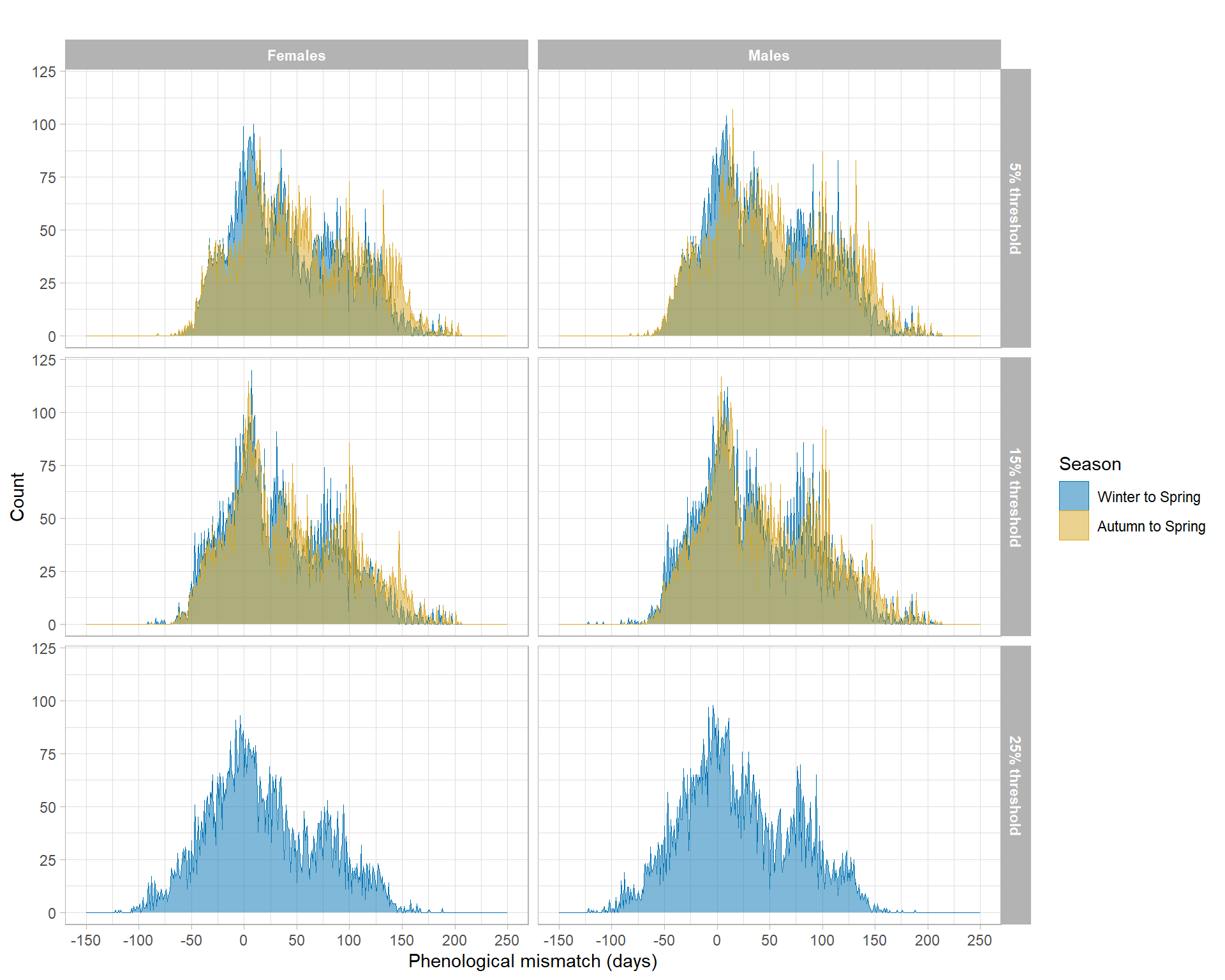
Phenological mismatches were visualized as overlapping binned area histograms. Panels are arranged by threshold definition and sex, while colors distinguish the two seasonal-window definitions.
```{r}
#| label: fig-phenological-mismatch
#| fig-width: 10
#| fig-height: 8
#| fig-cap: "Distribution of phenological mismatch values under alternative bloom-onset thresholds and seasonal-window definitions. Panels are faceted by threshold definition (rows) and sex (columns), and colors distinguish Winter–Spring versus Autumn–Spring seasonal windows. Mismatch is defined as the difference in days between laying date and estimated bloom onset."
#| code-fold: true
#| code-summary: "Show plotting code"
season_palette <- c(
  "Winter to Spring" = "#0072B2", # Blue
  "Autumn to Spring" = "#DAA520"  # Gold (Goldenrod)
)


# Map fill and color to 'Season'
mismatch_plot <- ggplot(combined_data, aes(x = Value,
                                          fill = Season,
                                          color = Season)) +

  geom_area(
    stat = "bin",
    binwidth = 1,
    position = "identity",
    alpha = 0.5, # Alpha is critical for seeing the overlap
    linewidth = 0
  ) +

  # Faceting remains the same (3 rows, 2 cols)
 facet_grid(Mismatch_Type ~ Sex_Label) +

 labs(
  title = "",
  x = "Phenological mismatch (days)",
  y = "Count"
 ) +

  # --- Use the new 2-color palette ---
 scale_fill_manual(
    name = "Season",
    values = season_palette,
    drop = FALSE
  ) +
  scale_color_manual(
    name = "Season",
    values = season_palette,
    drop = FALSE
  ) +

 theme_light() +

 scale_x_continuous(limits = c(-150, 250), breaks = seq(-150, 250, 50)) +

  theme(
  legend.position = "right",
    strip.text = element_text(face = "bold")
  )


print(mismatch_plot)
```
The figure provides a visual comparison of how mismatch distributions change under alternative bloom-onset definitions used in the sensitivity analyses. Differences among panels indicate how both threshold choice and seasonal-window definition can influence the estimated timing gap between breeding and marine productivity.
```{r}
#| label: save-mismatch-plot
#| eval: false
ggsave(filename = here("..","Plots", "mismatch_thresholds.pdf"),
       plot = mismatch_plot,
       dpi = 300, device = cairo_pdf)

ggsave(filename = here("..","Plots", "mismatch_thresholds.jpg"),
       plot = mismatch_plot,
       width = 9,
       height = 7,
       dpi = 300)
```
## Reproducibility
::: {.callout-tip appearance="simple" collapse="true"}
Session information
```{r}
#| echo: false
#| warning: false
#| message: false
utils::sessionInfo()
```
:::