Leave-one-out

To evaluate whether the overall meta-analytic estimate is driven by any single study, we perform a leave-one-out analysis at the study level.

For each iteration, we refit the full multilevel model after removing all effect sizes from one study and record the resulting overall lnRR estimate. If the pooled effect remains stable across iterations, this indicates that the main result is not unduly influenced by any single study.

db <- readr::read_csv(here("..","data","db_effect_sizes.csv")) %>%
mutate(across(c(C_n, Ex_n, C_mean, Ex_mean, C_SE, Ex_SE, C_SD, Ex_SD, lnRR, lnRR_var), as.numeric))%>%
  mutate(across(where(is.character), as.factor))




db <- db %>%
  mutate(Study = str_extract(Study_ID, ".*_\\d{4}"))

VCV <- metafor::vcalc(
  vi = lnRR_var,
  cluster = Cohort_ID, # The clustering variable (Study_ID + Ex_ID)
  obs = ES_ID,         # The unique observation/effect size ID
  rho = 0.5,           # Assumed correlation between outcomes from the same cohort
  data = db 
)

Because our model uses a variance–covariance matrix (VCV) to account for within-cohort dependence, we must recompute that matrix each time a study is removed. The vcalc_args object ensures that the same covariance structure (cluster variable and assumed correlation) is applied during each refitting step.

vcalc_args <- list(vi = "lnRR_var",
                   cluster = "Cohort_ID",
                   obs = "ES_ID",
                   rho = 0.5)

ma_all <- rma.mv(yi = lnRR,
                  V = VCV, 
                  random = list(~1 | Study_ID,
                                ~1 | ES_ID,
                                ~1 | Strain),
                  test = "t",
                  method = "REML", 
                  data = db)

summary(ma_all)

Multivariate Meta-Analysis Model (k = 298; method: REML)

   logLik   Deviance        AIC        BIC       AICc   
-242.8851   485.7702   493.7702   508.5452   493.9072   

Variance Components:

            estim    sqrt  nlvls  fixed    factor 
sigma^2.1  0.0494  0.2223     20     no  Study_ID 
sigma^2.2  0.2302  0.4798    298     no     ES_ID 
sigma^2.3  0.0000  0.0001      6     no    Strain 

Test for Heterogeneity:
Q(df = 297) = 5799.5331, p-val < .0001

Model Results:

estimate      se     tval   df    pval    ci.lb    ci.ub     
 -0.2120  0.0662  -3.2046  297  0.0015  -0.3422  -0.0818  ** 

---
Signif. codes:  0 '***' 0.001 '**' 0.01 '*' 0.05 '.' 0.1 ' ' 1

loo_t<-leave_one_out(ma_all, group = "Study", vcalc_args =vcalc_args)

loo_t

                 name   estimate    lowerCL     upperCL    lowerPR   upperPR
1  Krishnamurthy_2025 -0.1804714 -0.3067364 -0.05420638 -1.1310613 0.7701185
2        Freitas_2020 -0.2345608 -0.3662627 -0.10285889 -1.2898706 0.8207490
3        Saghari_2021 -0.2186383 -0.3569070 -0.08036970 -1.2871952 0.8499185
4      Escribano_2014 -0.1452226 -0.2177303 -0.07271486 -0.9724561 0.6820110
5    Papadakakis_2019 -0.2169011 -0.3567353 -0.07706679 -1.3045233 0.8707212
6             Fu_2023 -0.1993904 -0.3384132 -0.06036748 -1.2615261 0.8627454
7        Sampaio_2017 -0.2205727 -0.3622150 -0.07893040 -1.3101872 0.8690418
8             Fu_2025 -0.2184528 -0.3541891 -0.08271651 -1.2824768 0.8455712
9        Niehues_2011 -0.2185420 -0.3593437 -0.07774032 -1.2815548 0.8444707
10    Pangemanan_2024 -0.2078496 -0.3398487 -0.07585035 -1.2595242 0.8438251
11          Chen_2019 -0.2108857 -0.3478612 -0.07391022 -1.2811460 0.8593745
12           Ren_2024 -0.2076347 -0.3429355 -0.07233395 -1.2080585 0.7927891
13      Milbratz_2017 -0.2122834 -0.3504070 -0.07415990 -1.2868257 0.8622589
14        Flores_2018 -0.2227915 -0.3584293 -0.08715384 -1.2809836 0.8354005
15         Cheng_2024 -0.2126974 -0.3506180 -0.07477677 -1.2892410 0.8638462
16       Rizzolo_2021 -0.2132545 -0.3449213 -0.08158768 -1.2654004 0.8388914
17       Camargo_2013 -0.2126936 -0.3490734 -0.07631379 -1.2721668 0.8467797
18     Terzioglu_2020 -0.2175428 -0.3560578 -0.07902784 -1.2703522 0.8352666
19            Li_2010 -0.2216599 -0.3580481 -0.08527166 -1.2902300 0.8469103
20     Chikahisa_2007 -0.2220461 -0.3626064 -0.08148583 -1.3353737 0.8912814

loo_plot<-orchard_leave1out(leave1out = loo_t,
                  xlab = "lnRR",
                  ylab = "Studies left out",
                  trunk.size = 0.3,
                  branch.size = 2,
                  alpha = 0.3,
                  legend.pos = "top.out")


loo_plot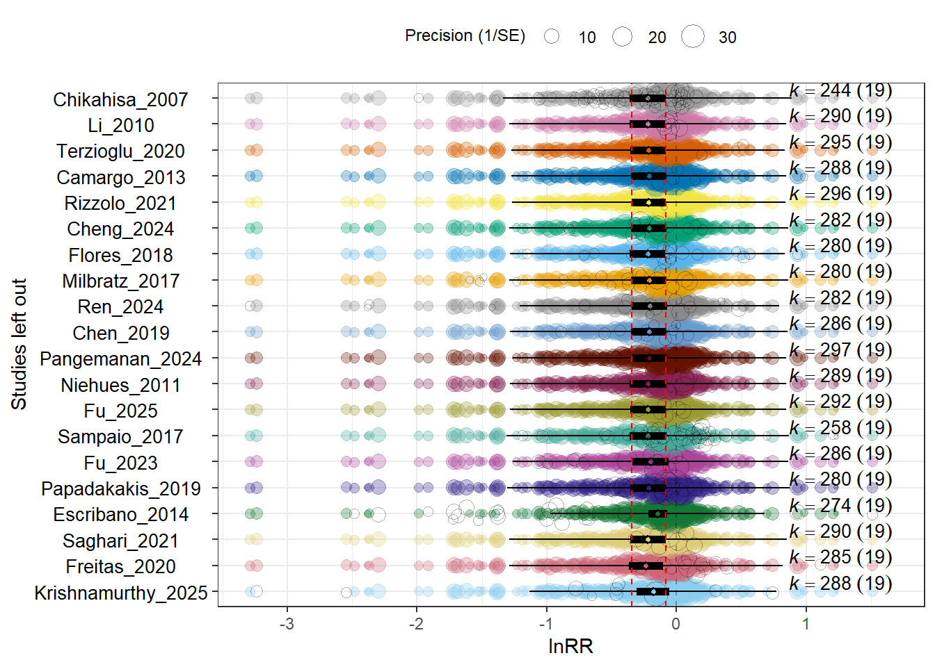

Across iterations, the pooled lnRR estimate remained within a narrow range and consistently below zero. No single study reversed the direction or substantially altered the magnitude of the overall effect. This indicates that the observed reduction in anxiety- and depression-like behaviors under music exposure is not driven by any individual dataset and is robust to study-level exclusion.

ggsave(filename = here("..","Plots", "loo_studies.pdf"),
       plot = loo_plot,
       dpi = 300, device = cairo_pdf,width = 12,  
       height = 10)

ggsave(filename = here("..","Plots", "loo_studies.jpg"),
       plot = loo_plot,
       width = 12,  
       height = 10,  
       dpi = 300)

Note

sessionInfo()

R version 4.5.2 (2025-10-31 ucrt)
Platform: x86_64-w64-mingw32/x64
Running under: Windows 11 x64 (build 26200)

Matrix products: default
  LAPACK version 3.12.1

locale:
[1] LC_COLLATE=English_Guernsey.utf8  LC_CTYPE=English_Guernsey.utf8   
[3] LC_MONETARY=English_Guernsey.utf8 LC_NUMERIC=C                     
[5] LC_TIME=English_Guernsey.utf8    

time zone: America/Edmonton
tzcode source: internal

attached base packages:
[1] stats     graphics  grDevices utils     datasets  methods   base     

other attached packages:
 [1] orchaRd_2.1.3       metafor_4.8-0       numDeriv_2016.8-1.1
 [4] metadat_1.4-0       Matrix_1.7-4        patchwork_1.3.2    
 [7] lubridate_1.9.4     forcats_1.0.1       stringr_1.6.0      
[10] dplyr_1.1.4         purrr_1.2.1         readr_2.1.6        
[13] tidyr_1.3.2         tibble_3.3.1        ggplot2_4.0.1      
[16] tidyverse_2.0.0     knitr_1.51          here_1.0.2         
[19] dtplyr_1.3.2        DT_0.34.0          

loaded via a namespace (and not attached):
 [1] beeswarm_0.4.0      gtable_0.3.6        xfun_0.56          
 [4] htmlwidgets_1.6.4   lattice_0.22-7      mathjaxr_2.0-0     
 [7] tzdb_0.5.0          vctrs_0.7.1         tools_4.5.2        
[10] generics_0.1.4      parallel_4.5.2      sandwich_3.1-1     
[13] pacman_0.5.1        pkgconfig_2.0.3     data.table_1.18.2.1
[16] RColorBrewer_1.1-3  S7_0.2.1            lifecycle_1.0.5    
[19] compiler_4.5.2      farver_2.1.2        codetools_0.2-20   
[22] vipor_0.4.7         htmltools_0.5.9     yaml_2.3.12        
[25] pillar_1.11.1       crayon_1.5.3        MASS_7.3-65        
[28] multcomp_1.4-29     nlme_3.1-168        tidyselect_1.2.1   
[31] digest_0.6.39       mvtnorm_1.3-3       stringi_1.8.7      
[34] labeling_0.4.3      splines_4.5.2       latex2exp_0.9.8    
[37] rprojroot_2.1.1     fastmap_1.2.0       grid_4.5.2         
[40] cli_3.6.5           magrittr_2.0.4      survival_3.8-6     
[43] TH.data_1.1-5       withr_3.0.2         scales_1.4.0       
[46] bit64_4.6.0-1       ggbeeswarm_0.7.3    timechange_0.3.0   
[49] estimability_1.5.1  rmarkdown_2.30      emmeans_2.0.1      
[52] bit_4.6.0           otel_0.2.0          zoo_1.8-15         
[55] hms_1.1.4           coda_0.19-4.1       evaluate_1.0.5     
[58] rlang_1.1.7         xtable_1.8-4        glue_1.8.0         
[61] rstudioapi_0.18.0   vroom_1.7.0         jsonlite_2.0.0     
[64] R6_2.6.1