---
title: "Publication bias"
---
First, we reload the data and run a simple intercept-only model (ma_all) to establish the overall mean effect size, which acts as the centerline for our funnel plots.
```{r}
#| label: setup
#|
pacman::p_load(
               DT,
               dtplyr,
               here,
               knitr,
               tidyverse,
               patchwork,
               metafor,
               orchaRd, emmeans,scales
               )
db <- readr::read_csv(here("..","data","db_effect_sizes.csv")) %>%
mutate(across( c(C_n, Ex_n, C_mean, Ex_mean, C_SE, Ex_SE, C_SD, Ex_SD, lnRR, lnRR_var), as.numeric))%>%
  mutate(across(where(is.character), as.factor))


VCV <- metafor::vcalc(
  vi = lnRR_var,
  cluster = Cohort_ID, # The clustering variable (Study_ID + Ex_ID)
  obs = ES_ID,         # The unique observation/effect size ID
  rho = 0.5,           # Assumed correlation between outcomes from the same cohort
  data = db
)

ma_all <- rma.mv(yi = lnRR,
                  V = VCV,
                  random = list(~1 | Study_ID,
                                ~1 | ES_ID,
                                ~1 | Strain),
                  test = "t",
                  method = "REML",
                  sparse = TRUE,
                  data = db)

summary(ma_all)
```
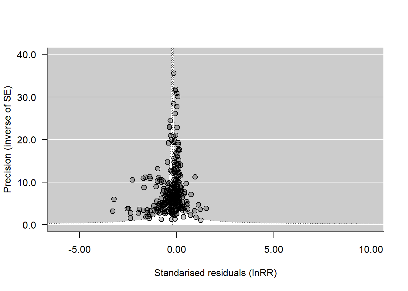
## Visual inspection: funnel plots
```{r}
#| label: funnel_plot
pdf(file = "funnel_plot.pdf", width = 8, height = 6)


funnel_plot <- funnel(ma_all,
       yaxis = "seinv",
       las = 1,
       digits = c(2, 1),
       xlab = "Standarised residuals (lnRR)",
       ylab = "Precision (inverse of SE)",
       pch = 21,
       bg = alpha("black", 0.2),
       col = "black",
       cex = 1.2,
       ylim = c(0.01, 40),
       xlim = c(-6, 10)
)


dev.off()
```
```{r}
#| label: funnel
#| echo: false
funnel_plot <- funnel(ma_all,
yaxis = "seinv",
las = 1,
digits = c(2, 1),
xlab = "Standarised residuals (lnRR)",
ylab = "Precision (inverse of SE)",
pch = 21,
bg = alpha("black", 0.2),
col = "black",
cex = 1.2,
ylim = c(0.01, 40),
xlim = c(-6, 10)
)
```
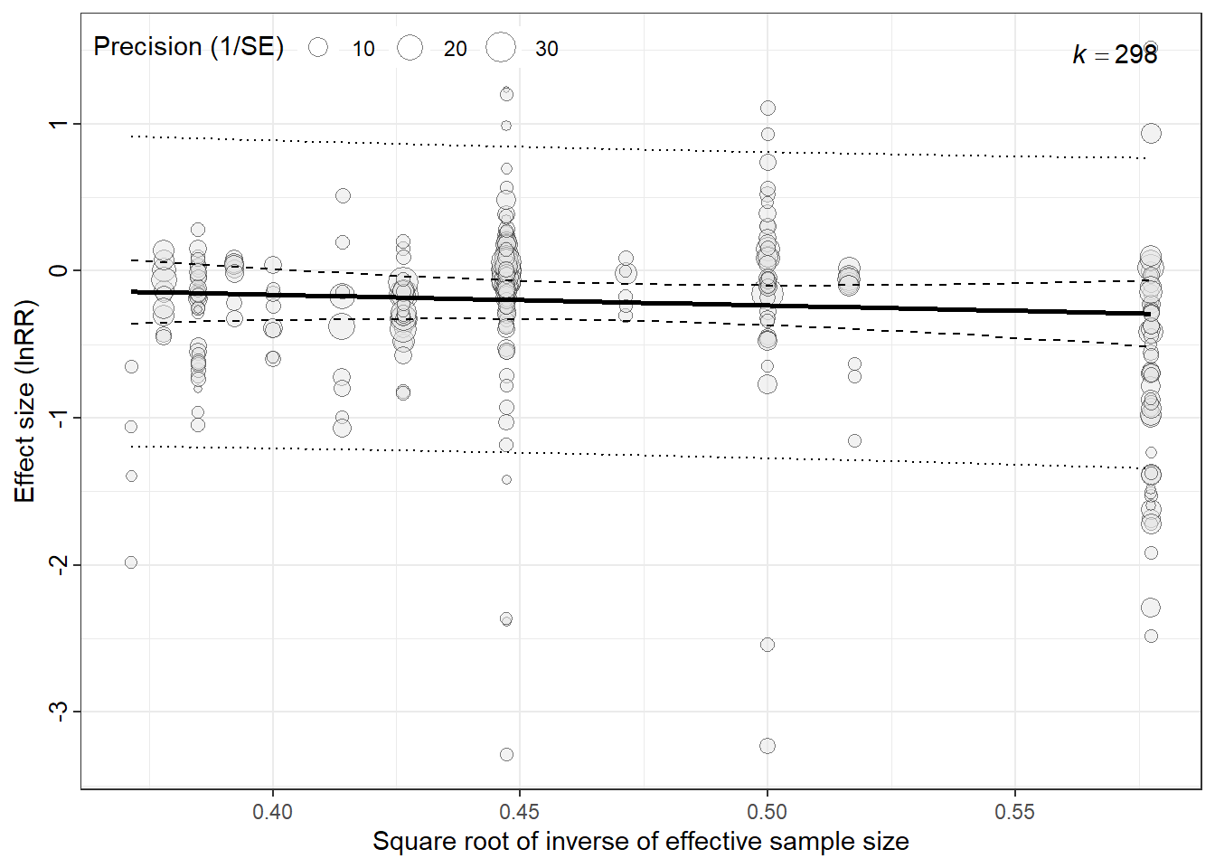
## Egger's Regression (Testing Small-Study Effects)
We tested for small-study effects using an Egger-type meta-regression adapted for lnRR. Because lnRR and its sampling variance are mathematically coupled, regressions on the standard error can be biased. Following recommendations for multilevel meta-analysis, we used an N-based precision proxy and fitted it as a moderator in the same multilevel model.
```{r}
#| label: eggers_test
# 1. Calculate the effective sample size term (sqrt_inv_e_n)
# Formula: sqrt(1/Ex_n + 1/C_n) approximates the standard error based on N
dt_egger_full <- db %>%
  mutate(sqrt_inv_e_n = sqrt((1 / Ex_n) + (1 / C_n)))

# 2. Run the Meta-Regression
# If 'sqrt_inv_e_n' is significant (p < 0.05), we have evidence of small-study effects.
egger_model_full <- rma.mv(yi = lnRR,
                           V = VCV,
                           mods = ~ 1 + sqrt_inv_e_n, # The 'Egger' predictor
                           random = list(~1 | Study_ID, ~1|Strain, ~1 | ES_ID),
                           test = "t",
                           method = "REML",
                           data = dt_egger_full)

summary(egger_model_full)
```
```{r}
#| label: egger_bubble_plot
egger<-bubble_plot(egger_model_full,
            mod = "sqrt_inv_e_n",
            group = "Study_ID",
            xlab = "Square root of inverse of effective sample size", ylab="Effect size (lnRR)")

egger
```
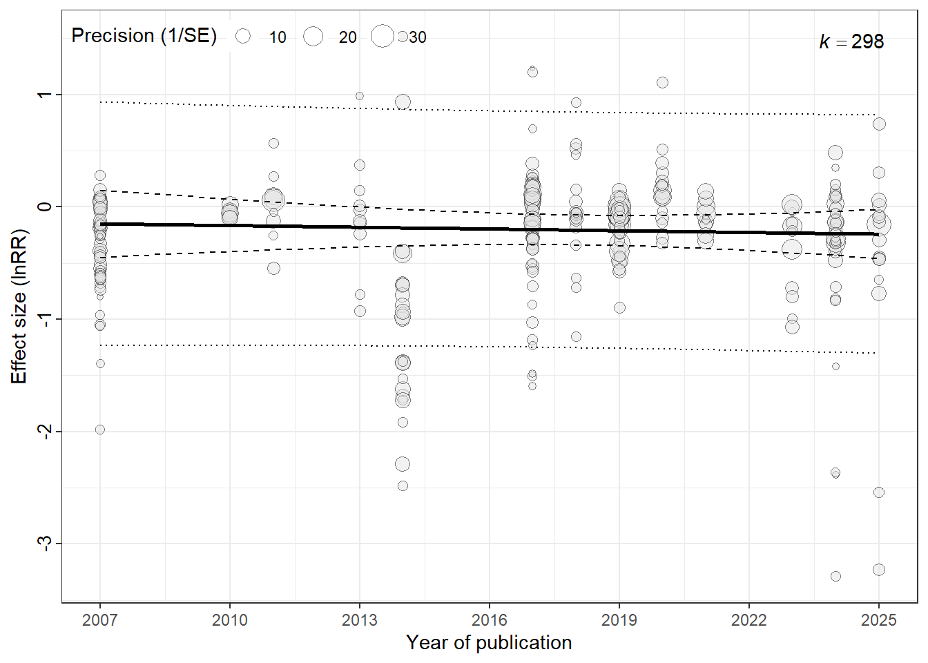
## Decline Effect (Time-Lag Bias)
Often in science, early studies show large effects (novelty bias), but as time goes on and methods improve (or replication attempts increase), the effect size shrinks. This is called the Decline Effect or Time-Lag Bias.
We test this by adding Publication Year to the model. A significant negative slope indicates the effect is shrinking over time.
```{r}
#| label: time_lag_analysis
# 1. Mean-Center the Year (Interpretation: Intercept = Effect in average year)
db_decline <- dt_egger_full %>%
  mutate(Year_c = Year - mean(Year, na.rm = TRUE))

# 2. Run model: Controlling for Precision (Egger) AND Year simultaneously
year_lag_model <- rma.mv(yi = lnRR,
                         V = VCV,
                         mods = ~ 1 + Year_c + sqrt_inv_e_n,
                         random = list(~1 | Study_ID, ~1|Strain,~1 | ES_ID),
                         test = "t",
                         method = "REML",
                         sparse = TRUE,
                         data = db_decline)

summary(year_lag_model)
```
```{r}
#| label: time_lag_bubble_plot
time_lag<-bubble_plot(year_lag_model,
            mod = "Year_c",
            group = "Study_ID",
            xlab = "Year of publication",ylab="Effect size (lnRR)")


mean_year <- mean(dt_egger_full$Year, na.rm = TRUE)

# Define the years you want to see on the axis
target_years <- seq(2007, 2025, by = 3)

lag2<-time_lag +
  scale_x_continuous(
    name = "Year of publication",
    breaks = target_years - mean_year,
    labels = target_years
  )

lag2
```
```{r}
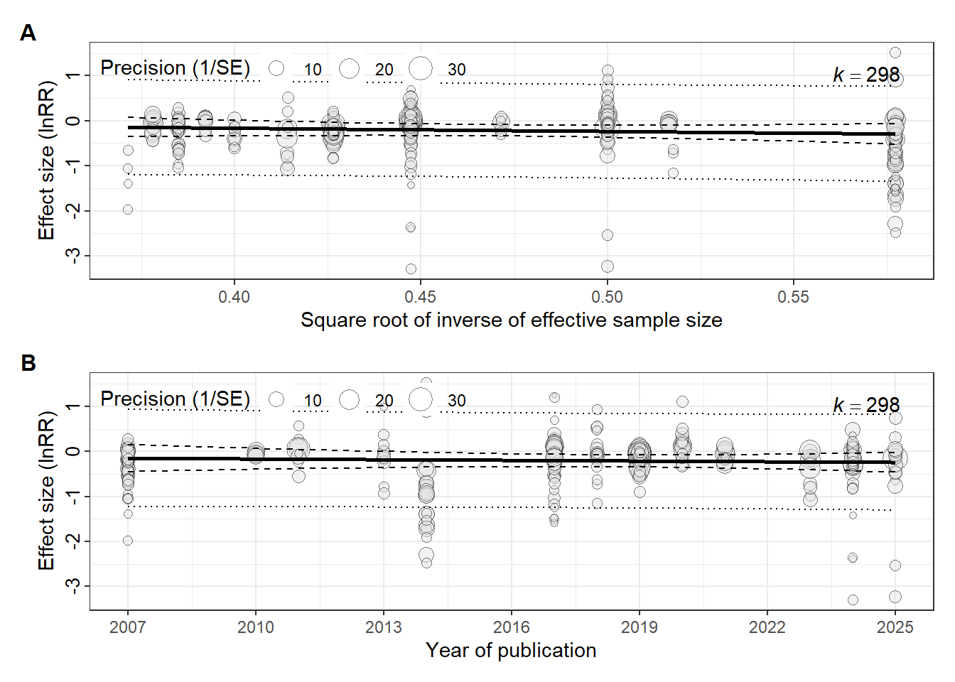
#| label: final_dashboard
final_dashboard <- egger / lag2 +
  plot_annotation(tag_levels = "A")  &
  theme(
    plot.tag = element_text(size = 12, face = "bold"),
    plot.subtitle = element_text(size = 10, face = "bold")
  )

final_dashboard
```
```{r}
#| label: save-figure_behaviour
#| eval: false
ggsave(filename = here("..","Plots", "bias_lnRR.pdf"),
       plot = final_dashboard,
       dpi = 300, device = cairo_pdf,width = 10,
       height = 7)

ggsave(filename = here("..","Plots", "bias_lnRR.jpg"),
       plot = final_dashboard,
       width = 10,
       height = 7,
       dpi = 300)
```
We treat all publication-bias diagnostics as exploratory because heterogeneity is high and effect sizes are dependent. We interpret agreement across the funnel plot, Egger-type regression, and the year moderator as stronger evidence than any single test.
::: callout-note
```{r}
sessionInfo()
```
:::