pacman::p_load(
  DT, dtplyr, here, knitr, tidyverse, patchwork, metafor, orchaRd, multcomp
)

db_all <- readr::read_csv(here("..","data","db_effect_sizes.csv")) %>%
  mutate(across(where(is.character), as.factor)) %>%
  mutate(across(c(lnRR, lnRR_var, lnVR, lnVR_var, lnCVR, lnCVR_var), as.numeric))%>%
  mutate(
    Control_conditions = as.character(Control_conditions),
    Control_conditions = dplyr::recode(
      Control_conditions,
      "ambiet sound" = "Ambient sound",
      "white noise"  = "White noise"
    ),
    Control_conditions = factor(Control_conditions)
  )

# Per-metric datasets
db_rr  <- db_all %>% filter(!is.na(lnRR),  !is.na(lnRR_var))
db_vr  <- db_all %>% filter(!is.na(lnVR),  !is.na(lnVR_var))
db_cvr <- db_all %>% filter(!is.na(lnCVR), !is.na(lnCVR_var))

# Per-metric VCV matrices (rho = 0.5)
VCV_rr <- metafor::vcalc(vi = lnRR_var,  cluster = Cohort_ID, obs = ES_ID, rho = 0.5, data = db_rr)
VCV_vr <- metafor::vcalc(vi = lnVR_var,  cluster = Cohort_ID, obs = ES_ID, rho = 0.5, data = db_vr)
VCV_cvr<- metafor::vcalc(vi = lnCVR_var, cluster = Cohort_ID, obs = ES_ID, rho = 0.5, data = db_cvr)Uni-moderators
We fit uni-moderator multilevel meta-regressions to test whether study characteristics predict differences in:
the mean response (lnRR),
absolute variability (lnVR),
relative variability (lnCVR).
Each moderator is analysed separately (uni-moderator), using the same random-effects structure (Study_ID, ES_ID, Strain`) and a cohort-level VCV matrix (rho = 0.5). For categorical moderators, we drop levels with fewer than five effect sizes (k < 5) within each effect size metric, and subset the corresponding VCV matrix accordingly.
NoteHelper functions
Filter to common moderator levels (k ≥ 5 in each metric)
Code
filter_low_k_single <- function(dat, V, moderator, min_k = 5) {
  mod_chr <- moderator
  # If moderator is not a factor, just return as-is
  if (!is.factor(dat[[mod_chr]])) {
    return(list(data = dat, V = V, keep_levels = NULL, k = NULL))
  }

  k_counts <- dat %>%
    count(.data[[mod_chr]], name = "k_es")

  keep_levels <- k_counts %>%
    filter(k_es >= min_k) %>%
    pull(.data[[mod_chr]])

  dat_f <- dat %>% filter(.data[[mod_chr]] %in% keep_levels)
  idx   <- which(dat[[mod_chr]] %in% keep_levels)
  V_f   <- V[idx, idx, drop = FALSE]

  list(data = dat_f, V = V_f, keep_levels = keep_levels, k = k_counts)
}
Fit one uni-moderator model + plot
Code
fit_unimod <- function(dat, V, yi, mods_formula, mod_name, xlab_expr) {

  # Guard: if nothing left after filtering
  if (nrow(dat) < 2) return(NULL)

  mod <- metafor::rma.mv(
    yi = dat[[yi]],
    V  = V,
    mods = as.formula(mods_formula),
    random = list(~1 | Study_ID, ~1 | ES_ID, ~1 | Strain),
    test = "t",
    method = "REML",
    sparse = TRUE,
    data = dat
  )

  list(
    data  = dat,
    model = mod,
    r2    = round(orchaRd::r2_ml(mod), 4),
    i2    = orchaRd::i2_ml(mod),
    plot  = orchard_plot(
      mod,
      mod   = mod_name,
      group = "Study_ID",
      xlab  = xlab_expr,
      flip  = TRUE,
      legend.pos  = "top.left",
      trunk.size  = 0.3,
      branch.size = 2,
      alpha       = 0.3
    ) +
      scale_colour_brewer(palette = "Set1") +
      scale_fill_brewer(palette = "Dark2") +
      theme(legend.direction = "vertical")
  )
}
Optional Tukey contrasts
Code
maybe_tukey <- function(dat, V, yi, moderator, min_k = 3) {

  dat <- dat %>%
    mutate("{moderator}" := droplevels(as.factor(.data[[moderator]])))

  k <- nlevels(dat[[moderator]])
  if (is.na(k) || k < min_k) return(NULL)

  # Fit without intercept so coef = one per level
  mods_formula <- as.formula(paste0("~ ", moderator, " - 1"))

  m <- metafor::rma.mv(
    yi = dat[[yi]],
    V  = V,
    mods = mods_formula,
    random = list(~1 | Study_ID,
                  ~1 | ES_ID,
                  ~1 | Strain),
    test = "t",
    method = "REML",
    sparse = TRUE,
    data = dat
  )

  cn <- names(coef(m))
  K <- multcomp::contrMat(rep(1, k), type = "Tukey")
  colnames(K) <- cn

  g <- multcomp::glht(m, linfct = K)


  base::summary(g, test = multcomp::adjusted("none"))
}
Outcome type
MOD  <- "Outcome_type"
MODS <- "~ Outcome_type"

f_rr  <- filter_low_k_single(db_rr,  VCV_rr,  MOD, min_k = 5)
f_vr  <- filter_low_k_single(db_vr,  VCV_vr,  MOD, min_k = 5)
f_cvr <- filter_low_k_single(db_cvr, VCV_cvr, MOD, min_k = 5)

res_rr  <- fit_unimod(f_rr$data,  f_rr$V,  "lnRR",  MODS, MOD, expression(lnRR))
res_vr  <- fit_unimod(f_vr$data,  f_vr$V,  "lnVR",  MODS, MOD, expression(lnVR))
res_cvr <- fit_unimod(f_cvr$data, f_cvr$V, "lnCVR", MODS, MOD, expression(lnCVR))
lnRR
summary(res_rr$model)
Multivariate Meta-Analysis Model (k = 295; method: REML)

   logLik   Deviance        AIC        BIC       AICc
-241.0967   482.1933   492.1933   510.5942   492.4024

Variance Components:

            estim    sqrt  nlvls  fixed    factor
sigma^2.1  0.0495  0.2225     20     no  Study_ID
sigma^2.2  0.2333  0.4830    295     no     ES_ID
sigma^2.3  0.0000  0.0000      6     no    Strain

Test for Residual Heterogeneity:
QE(df = 293) = 5690.1059, p-val < .0001

Test of Moderators (coefficient 2):
F(df1 = 1, df2 = 293) = 0.0236, p-val = 0.8781

Model Results:

                        estimate      se     tval   df    pval    ci.lb
intrcpt                  -0.2158  0.0710  -3.0389  293  0.0026  -0.3555
Outcome_typeDepression    0.0139  0.0907   0.1535  293  0.8781  -0.1645
                          ci.ub
intrcpt                 -0.0760  **
Outcome_typeDepression   0.1923

---
Signif. codes: 0 '***' 0.001 '**' 0.01 '*' 0.05 '.' 0.1 ' ' 1res_rr$r2 R2_marginal R2_conditional
0.0001 0.1752 res_rr$plot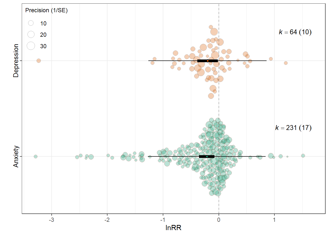
lnVR
summary(res_vr$model)
Multivariate Meta-Analysis Model (k = 219; method: REML)

   logLik   Deviance        AIC        BIC       AICc
-339.3184   678.6368   688.6368   705.5363   688.9211

Variance Components:

            estim    sqrt  nlvls  fixed    factor
sigma^2.1  0.1310  0.3620     16     no  Study_ID
sigma^2.2  1.1825  1.0874    219     no     ES_ID
sigma^2.3  0.0000  0.0001      6     no    Strain

Test for Residual Heterogeneity:
QE(df = 217) = 4218.8132, p-val < .0001

Test of Moderators (coefficient 2):
F(df1 = 1, df2 = 217) = 8.3073, p-val = 0.0043

Model Results:

                        estimate      se     tval   df    pval    ci.lb
intrcpt                   0.3112  0.1520   2.0473  217  0.0418   0.0116
Outcome_typeDepression   -0.6401  0.2221  -2.8822  217  0.0043  -1.0779
                          ci.ub
intrcpt                  0.6107   *
Outcome_typeDepression  -0.2024  **

---
Signif. codes: 0 '***' 0.001 '**' 0.01 '*' 0.05 '.' 0.1 ' ' 1res_vr$r2 R2_marginal R2_conditional
0.0537 0.1481 res_vr$plot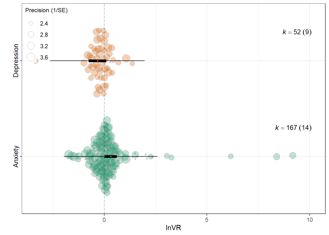
lnCVR
summary(res_cvr$model)
Multivariate Meta-Analysis Model (k = 219; method: REML)

   logLik   Deviance        AIC        BIC       AICc
-279.5331   559.0662   569.0662   585.9656   569.3505

Variance Components:

            estim    sqrt  nlvls  fixed    factor
sigma^2.1  0.1050  0.3240     16     no  Study_ID
sigma^2.2  0.5956  0.7718    219     no     ES_ID
sigma^2.3  0.0000  0.0000      6     no    Strain

Test for Residual Heterogeneity:
QE(df = 217) = 1576.9857, p-val < .0001

Test of Moderators (coefficient 2):
F(df1 = 1, df2 = 217) = 1.1590, p-val = 0.2829

Model Results:

                        estimate      se     tval   df    pval    ci.lb   ci.ub
intrcpt                   0.0615  0.1339   0.4590  217  0.6467  -0.2025  0.3255
Outcome_typeDepression   -0.1830  0.1700  -1.0766  217  0.2829  -0.5180  0.1520

intrcpt
Outcome_typeDepression

---
Signif. codes: 0 '***' 0.001 '**' 0.01 '*' 0.05 '.' 0.1 ' ' 1res_cvr$r2 R2_marginal R2_conditional
0.0086 0.1572 res_cvr$plot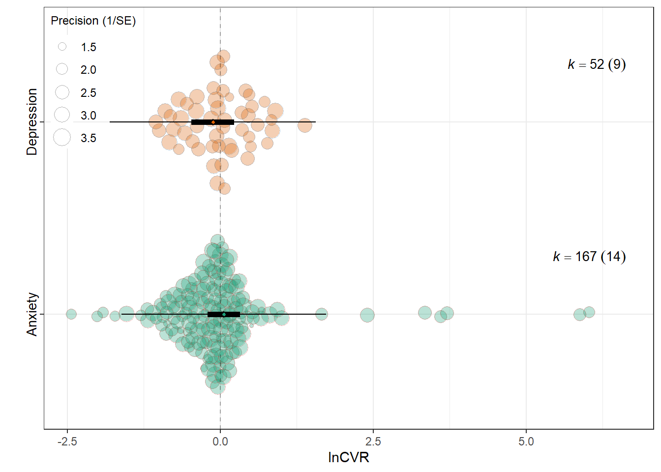
Behavioral assay
MOD  <- "Assay_type"
MODS <- "~ Assay_type - 1"


assay_labels <- c(
  "Elevated Plus Maze" = "EPM",
  "Open Field Test" = "OFT",
  "Light-Dark Box" = "LDB",
  "Forced Swim Test (FST)" = "FST",
  "Tail Suspension Test (TST)" = "TST",
  "Sucrose Preference Test (SPT)" = "SPT"
)


# 1) Filter each effect-size dataset (and subset the VCV accordingly)
f_rr  <- filter_low_k_single(db_rr,  VCV_rr,  MOD, min_k = 5)
f_vr  <- filter_low_k_single(db_vr,  VCV_vr,  MOD, min_k = 5)
f_cvr <- filter_low_k_single(db_cvr, VCV_cvr, MOD, min_k = 5)
# 2) Fit the three unimoderator models (same moderator, different yi/vi)
res_rr  <- fit_unimod(f_rr$data,  f_rr$V,  "lnRR",  MODS, MOD, expression(lnRR))
res_vr  <- fit_unimod(f_vr$data,  f_vr$V,  "lnVR",  MODS, MOD, expression(lnVR))
res_cvr <- fit_unimod(f_cvr$data, f_cvr$V, "lnCVR", MODS, MOD, expression(lnCVR))

# 2b) Relabel x-axis in the orchard plots (so EPM/OFT/etc. show)
res_rr$plot  <- res_rr$plot  + scale_x_discrete(labels = assay_labels)
res_vr$plot  <- res_vr$plot  + scale_x_discrete(labels = assay_labels)
res_cvr$plot <- res_cvr$plot + scale_x_discrete(labels = assay_labels)

# 3) Tukey contrasts (use the filtered data + matched VCV for each dataset)

tuk_rr  <- maybe_tukey(dat = f_rr$data,  V = f_rr$V,  yi = "lnRR",  moderator = MOD)
tuk_vr  <- maybe_tukey(dat = f_vr$data,  V = f_vr$V,  yi = "lnVR",  moderator = MOD)
tuk_cvr <- maybe_tukey(dat = f_cvr$data, V = f_cvr$V, yi = "lnCVR", moderator = MOD)
lnRR
summary(res_rr$model)
Multivariate Meta-Analysis Model (k = 289; method: REML)

   logLik   Deviance        AIC        BIC       AICc
-227.2656   454.5311   472.5311   505.3401   473.1904

Variance Components:

            estim    sqrt  nlvls  fixed    factor
sigma^2.1  0.0311  0.1763     20     no  Study_ID
sigma^2.2  0.2267  0.4762    289     no     ES_ID
sigma^2.3  0.0043  0.0654      6     no    Strain

Test for Residual Heterogeneity:
QE(df = 283) = 5482.7134, p-val < .0001

Test of Moderators (coefficients 1:6):
F(df1 = 6, df2 = 283) = 3.8229, p-val = 0.0011

Model Results:

                                         estimate      se     tval   df    pval
Assay_typeElevated Plus Maze              -0.2884  0.0805  -3.5807  283  0.0004
Assay_typeForced Swim Test (FST)          -0.3122  0.1127  -2.7713  283  0.0060
Assay_typeLight-Dark Box                  -0.5634  0.1518  -3.7114  283  0.0002
Assay_typeOpen Field Test                 -0.0699  0.0844  -0.8280  283  0.4084
Assay_typeSucrose Preference Test (SPT)   -0.0715  0.1574  -0.4542  283  0.6500
Assay_typeTail Suspension Test (TST)      -0.0926  0.2025  -0.4571  283  0.6480
                                           ci.lb    ci.ub
Assay_typeElevated Plus Maze             -0.4469  -0.1298  ***
Assay_typeForced Swim Test (FST)         -0.5339  -0.0905   **
Assay_typeLight-Dark Box                 -0.8622  -0.2646  ***
Assay_typeOpen Field Test                -0.2360   0.0963
Assay_typeSucrose Preference Test (SPT)  -0.3813   0.2383
Assay_typeTail Suspension Test (TST)     -0.4912   0.3061

---
Signif. codes: 0 '***' 0.001 '**' 0.01 '*' 0.05 '.' 0.1 ' ' 1res_rr$r2 R2_marginal R2_conditional
0.0709 0.1963 res_rr$plot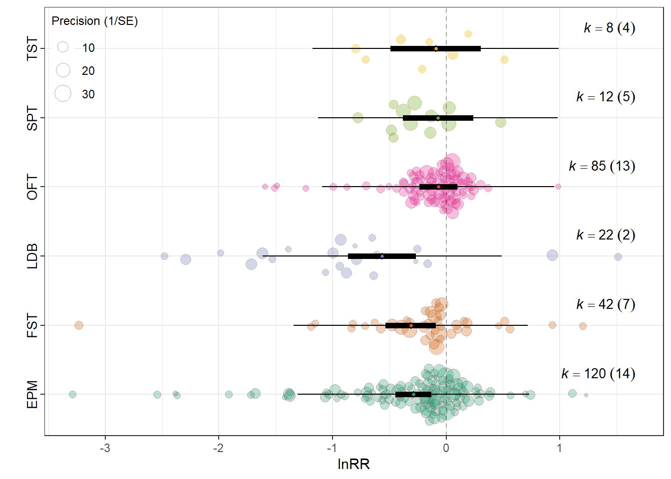
tuk_rr
     Simultaneous Tests for General Linear Hypotheses

Multiple Comparisons of Means: Tukey Contrasts


Fit: metafor::rma.mv(yi = dat[[yi]], V = V, mods = mods_formula, data = dat,
    random = list(~1 | Study_ID, ~1 | ES_ID, ~1 | Strain), method = "REML",
    test = "t", sparse = TRUE)

Linear Hypotheses:
            Estimate Std. Error z value Pr(>|z|)
2 - 1 == 0 -0.023825   0.112008  -0.213  0.83155
3 - 1 == 0 -0.275002   0.136691  -2.012  0.04424 *
4 - 1 == 0  0.218483   0.083046   2.631  0.00852 **
5 - 1 == 0  0.216889   0.162745   1.333  0.18263
6 - 1 == 0  0.195807   0.207107   0.945  0.34443
3 - 2 == 0 -0.251177   0.172914  -1.453  0.14633
4 - 2 == 0  0.242308   0.119213   2.033  0.04210 *
5 - 2 == 0  0.240714   0.179481   1.341  0.17987
6 - 2 == 0  0.219632   0.221942   0.990  0.32237
4 - 3 == 0  0.493485   0.153496   3.215  0.00130 **
5 - 3 == 0  0.491891   0.208187   2.363  0.01814 *
6 - 3 == 0  0.470809   0.244179   1.928  0.05384 .
5 - 4 == 0 -0.001594   0.163517  -0.010  0.99222
6 - 4 == 0 -0.022676   0.206881  -0.110  0.91272
6 - 5 == 0 -0.021082   0.243796  -0.086  0.93109
---
Signif. codes:  0 '***' 0.001 '**' 0.01 '*' 0.05 '.' 0.1 ' ' 1
(Adjusted p values reported -- none method)
lnVR
summary(res_vr$model)
Multivariate Meta-Analysis Model (k = 213; method: REML)

   logLik   Deviance        AIC        BIC       AICc
-321.7773   643.5546   659.5546   686.2549   660.2783

Variance Components:

            estim    sqrt  nlvls  fixed    factor
sigma^2.1  0.1545  0.3931     16     no  Study_ID
sigma^2.2  1.1373  1.0665    213     no     ES_ID
sigma^2.3  0.0000  0.0001      6     no    Strain

Test for Residual Heterogeneity:
QE(df = 208) = 3885.5939, p-val < .0001

Test of Moderators (coefficients 1:5):
F(df1 = 5, df2 = 208) = 4.4278, p-val = 0.0007

Model Results:

                                      estimate      se     tval   df    pval
Assay_typeElevated Plus Maze            0.7333  0.1947   3.7653  208  0.0002
Assay_typeForced Swim Test (FST)       -0.1735  0.2472  -0.7019  208  0.4835
Assay_typeLight-Dark Box                0.1806  0.3190   0.5659  208  0.5720
Assay_typeOpen Field Test              -0.0219  0.1924  -0.1138  208  0.9095
Assay_typeTail Suspension Test (TST)   -0.5177  0.4369  -1.1850  208  0.2374
                                        ci.lb   ci.ub
Assay_typeElevated Plus Maze           0.3493  1.1172  ***
Assay_typeForced Swim Test (FST)      -0.6609  0.3139
Assay_typeLight-Dark Box              -0.4484  0.8095
Assay_typeOpen Field Test             -0.4011  0.3573
Assay_typeTail Suspension Test (TST)  -1.3789  0.3436

---
Signif. codes: 0 '***' 0.001 '**' 0.01 '*' 0.05 '.' 0.1 ' ' 1res_vr$r2 R2_marginal R2_conditional
0.1119 0.2181 res_vr$plot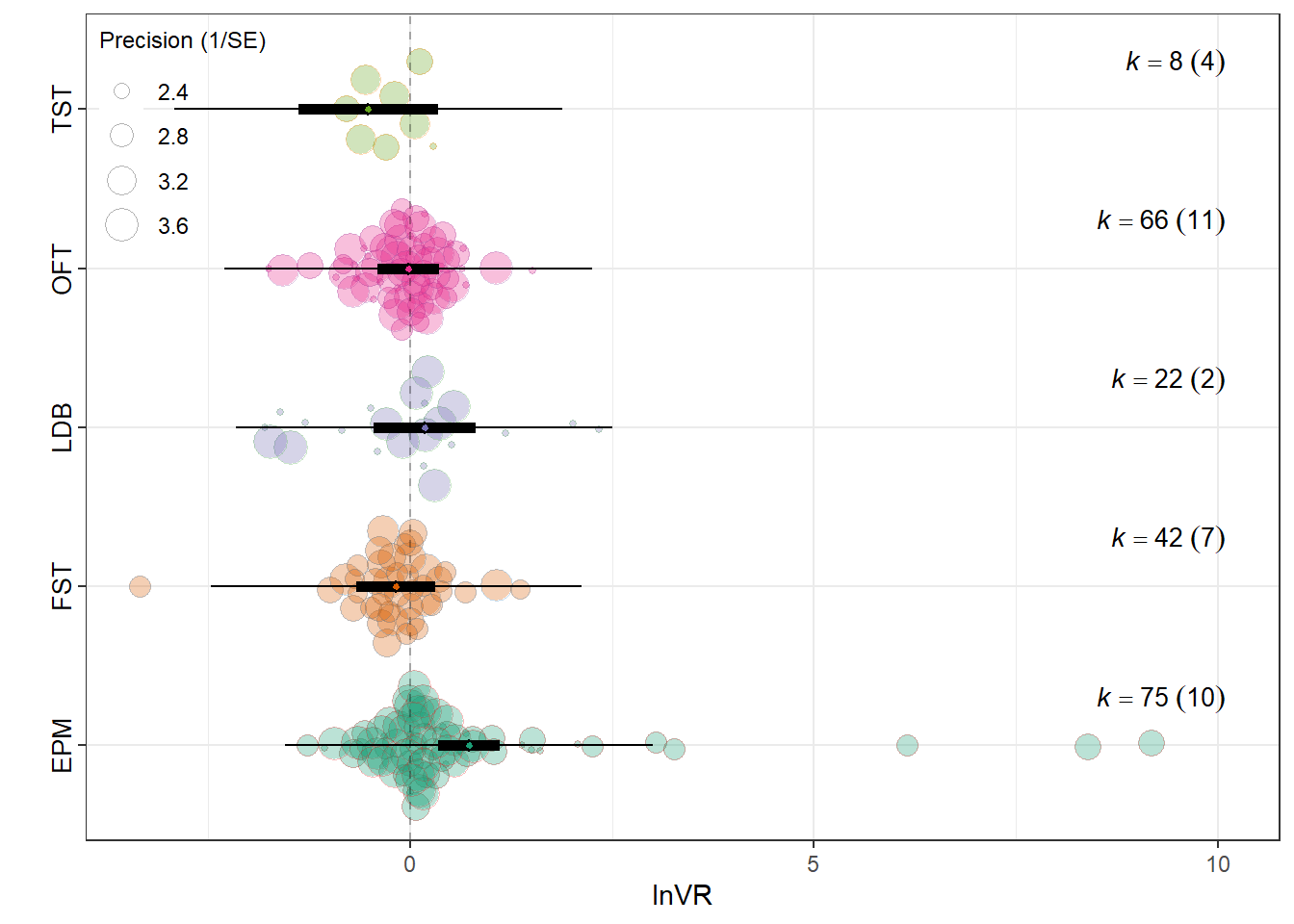
tuk_vr
     Simultaneous Tests for General Linear Hypotheses

Multiple Comparisons of Means: Tukey Contrasts


Fit: metafor::rma.mv(yi = dat[[yi]], V = V, mods = mods_formula, data = dat,
    random = list(~1 | Study_ID, ~1 | ES_ID, ~1 | Strain), method = "REML",
    test = "t", sparse = TRUE)

Linear Hypotheses:
           Estimate Std. Error z value Pr(>|z|)
2 - 1 == 0  -0.9068     0.2687  -3.375 0.000739 ***
3 - 1 == 0  -0.5527     0.2909  -1.900 0.057391 .
4 - 1 == 0  -0.7552     0.2241  -3.369 0.000754 ***
5 - 1 == 0  -1.2510     0.4611  -2.713 0.006670 **
3 - 2 == 0   0.3541     0.3775   0.938 0.348283
4 - 2 == 0   0.1516     0.2743   0.553 0.580379
5 - 2 == 0  -0.3442     0.4877  -0.706 0.480382
4 - 3 == 0  -0.2024     0.3416  -0.593 0.553443
5 - 3 == 0  -0.6982     0.5292  -1.319 0.187032
5 - 4 == 0  -0.4958     0.4573  -1.084 0.278306
---
Signif. codes:  0 '***' 0.001 '**' 0.01 '*' 0.05 '.' 0.1 ' ' 1
(Adjusted p values reported -- none method)
lnCVR
summary(res_cvr$model)
Multivariate Meta-Analysis Model (k = 213; method: REML)

   logLik   Deviance        AIC        BIC       AICc
-267.8978   535.7956   551.7956   578.4959   552.5192

Variance Components:

            estim    sqrt  nlvls  fixed    factor
sigma^2.1  0.1244  0.3526     16     no  Study_ID
sigma^2.2  0.5920  0.7694    213     no     ES_ID
sigma^2.3  0.0000  0.0000      6     no    Strain

Test for Residual Heterogeneity:
QE(df = 208) = 1504.7562, p-val < .0001

Test of Moderators (coefficients 1:5):
F(df1 = 5, df2 = 208) = 1.1484, p-val = 0.3360

Model Results:

                                      estimate      se     tval   df    pval
Assay_typeElevated Plus Maze            0.2586  0.1667   1.5511  208  0.1224
Assay_typeForced Swim Test (FST)       -0.0550  0.2029  -0.2709  208  0.7867
Assay_typeLight-Dark Box                0.1576  0.2660   0.5924  208  0.5543
Assay_typeOpen Field Test              -0.1324  0.1622  -0.8164  208  0.4152
Assay_typeTail Suspension Test (TST)   -0.1191  0.3430  -0.3473  208  0.7287
                                        ci.lb   ci.ub
Assay_typeElevated Plus Maze          -0.0701  0.5872
Assay_typeForced Swim Test (FST)      -0.4550  0.3451
Assay_typeLight-Dark Box              -0.3669  0.6820
Assay_typeOpen Field Test             -0.4521  0.1873
Assay_typeTail Suspension Test (TST)  -0.7953  0.5571

---
Signif. codes: 0 '***' 0.001 '**' 0.01 '*' 0.05 '.' 0.1 ' ' 1res_cvr$r2 R2_marginal R2_conditional
0.0405 0.2070 res_cvr$plot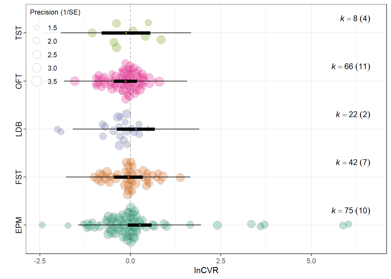
tuk_cvr
     Simultaneous Tests for General Linear Hypotheses

Multiple Comparisons of Means: Tukey Contrasts


Fit: metafor::rma.mv(yi = dat[[yi]], V = V, mods = mods_formula, data = dat,
    random = list(~1 | Study_ID, ~1 | ES_ID, ~1 | Strain), method = "REML",
    test = "t", sparse = TRUE)

Linear Hypotheses:
           Estimate Std. Error z value Pr(>|z|)
2 - 1 == 0 -0.31354    0.20741  -1.512   0.1306
3 - 1 == 0 -0.10099    0.22731  -0.444   0.6568
4 - 1 == 0 -0.39097    0.17392  -2.248   0.0246 *
5 - 1 == 0 -0.37769    0.35917  -1.052   0.2930
3 - 2 == 0  0.21255    0.29885   0.711   0.4769
4 - 2 == 0 -0.07743    0.21225  -0.365   0.7153
5 - 2 == 0 -0.06415    0.37941  -0.169   0.8657
4 - 3 == 0 -0.28998    0.27232  -1.065   0.2869
5 - 3 == 0 -0.27670    0.41692  -0.664   0.5069
5 - 4 == 0  0.01329    0.35474   0.037   0.9701
---
Signif. codes:  0 '***' 0.001 '**' 0.01 '*' 0.05 '.' 0.1 ' ' 1
(Adjusted p values reported -- none method)
Behavioral mechanism
MOD  <- "Induced behaviour"
MODS <- "~ `Induced behaviour`"

f_rr  <- filter_low_k_single(db_rr,  VCV_rr,  MOD, min_k = 5)
f_vr  <- filter_low_k_single(db_vr,  VCV_vr,  MOD, min_k = 5)
f_cvr <- filter_low_k_single(db_cvr, VCV_cvr, MOD, min_k = 5)

res_rr  <- fit_unimod(f_rr$data,  f_rr$V,  "lnRR",  MODS, MOD, expression(lnRR))
res_vr  <- fit_unimod(f_vr$data,  f_vr$V,  "lnVR",  MODS, MOD, expression(lnVR))
res_cvr <- fit_unimod(f_cvr$data, f_cvr$V, "lnCVR", MODS, MOD, expression(lnCVR))
lnRR
summary(res_rr$model)
Multivariate Meta-Analysis Model (k = 298; method: REML)

   logLik   Deviance        AIC        BIC       AICc
-238.1126   476.2252   486.2252   504.6770   486.4321

Variance Components:

            estim    sqrt  nlvls  fixed    factor
sigma^2.1  0.0484  0.2199     20     no  Study_ID
sigma^2.2  0.2228  0.4720    298     no     ES_ID
sigma^2.3  0.0000  0.0001      6     no    Strain

Test for Residual Heterogeneity:
QE(df = 296) = 5461.1248, p-val < .0001

Test of Moderators (coefficient 2):
F(df1 = 1, df2 = 296) = 8.4650, p-val = 0.0039

Model Results:

                           estimate      se     tval   df    pval    ci.lb
intrcpt                     -0.4579  0.1072  -4.2731  296  <.0001  -0.6688
`Induced behaviour`Innate    0.3222  0.1107   2.9095  296  0.0039   0.1043
                             ci.ub
intrcpt                    -0.2470  ***
`Induced behaviour`Innate   0.5401   **

---
Signif. codes: 0 '***' 0.001 '**' 0.01 '*' 0.05 '.' 0.1 ' ' 1res_rr$r2 R2_marginal R2_conditional
0.0524 0.2214 res_rr$plot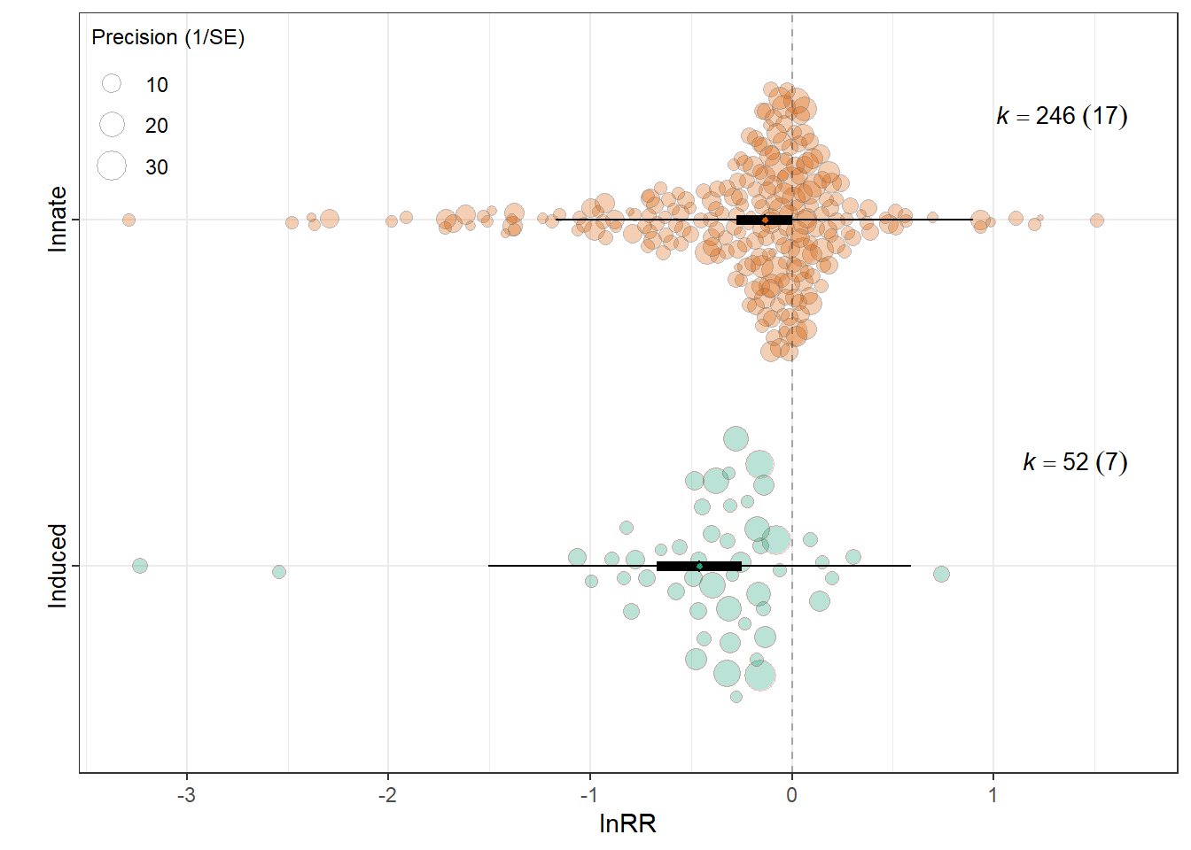
lnVR
summary(res_vr$model)
Multivariate Meta-Analysis Model (k = 222; method: REML)

   logLik   Deviance        AIC        BIC       AICc
-346.5856   693.1713   703.1713   720.1394   703.4517

Variance Components:

            estim    sqrt  nlvls  fixed    factor
sigma^2.1  0.0926  0.3043     16     no  Study_ID
sigma^2.2  1.2261  1.1073    222     no     ES_ID
sigma^2.3  0.0000  0.0001      6     no    Strain

Test for Residual Heterogeneity:
QE(df = 220) = 4389.9716, p-val < .0001

Test of Moderators (coefficient 2):
F(df1 = 1, df2 = 220) = 0.2942, p-val = 0.5881

Model Results:

                           estimate      se     tval   df    pval    ci.lb
intrcpt                      0.2494  0.2478   1.0064  220  0.3153  -0.2390
`Induced behaviour`Innate   -0.1461  0.2694  -0.5424  220  0.5881  -0.6771
                            ci.ub
intrcpt                    0.7378
`Induced behaviour`Innate  0.3848

---
Signif. codes: 0 '***' 0.001 '**' 0.01 '*' 0.05 '.' 0.1 ' ' 1res_vr$r2 R2_marginal R2_conditional
0.0022 0.0723 res_vr$plot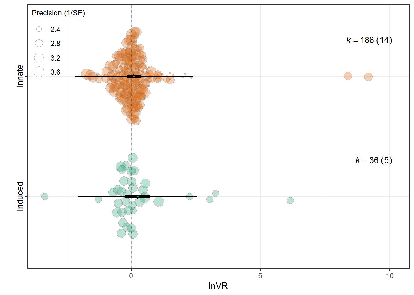
lnCVR
summary(res_cvr$model)
Multivariate Meta-Analysis Model (k = 222; method: REML)

   logLik   Deviance        AIC        BIC       AICc
-282.2780   564.5560   574.5560   591.5241   574.8364

Variance Components:

            estim    sqrt  nlvls  fixed    factor
sigma^2.1  0.0766  0.2768     16     no  Study_ID
sigma^2.2  0.5953  0.7715    222     no     ES_ID
sigma^2.3  0.0000  0.0000      6     no    Strain

Test for Residual Heterogeneity:
QE(df = 220) = 1588.3881, p-val < .0001

Test of Moderators (coefficient 2):
F(df1 = 1, df2 = 220) = 0.5346, p-val = 0.4655

Model Results:

                           estimate      se     tval   df    pval    ci.lb
intrcpt                      0.1362  0.2021   0.6741  220  0.5010  -0.2621
`Induced behaviour`Innate   -0.1563  0.2138  -0.7311  220  0.4655  -0.5777
                            ci.ub
intrcpt                    0.5345
`Induced behaviour`Innate  0.2651

---
Signif. codes: 0 '***' 0.001 '**' 0.01 '*' 0.05 '.' 0.1 ' ' 1res_cvr$r2 R2_marginal R2_conditional
0.0049 0.1184 res_cvr$plot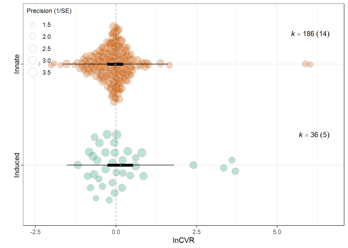
Lifestage of exposure
MOD  <- "Lifestage_exposure"
MODS <- "~ Lifestage_exposure -1"


lifestage_labels <- c(
  "Adolescent"  = "Adol.",
  "Adult"       = "Adult",
  "Juvenile"    = "Juv.",
  "Young adult" = "Y. adult",
  "Mixed"       = "Mixed",
  "Unclear"     = "Unclear"
)


# 1) Filter each effect-size dataset (and subset the VCV accordingly)
f_rr  <- filter_low_k_single(db_rr,  VCV_rr,  MOD, min_k = 5)
f_vr  <- filter_low_k_single(db_vr,  VCV_vr,  MOD, min_k = 5)
f_cvr <- filter_low_k_single(db_cvr, VCV_cvr, MOD, min_k = 5)


# 2) Fit the three unimoderator models (same moderator, different yi/vi)
res_rr  <- fit_unimod(f_rr$data,  f_rr$V,  "lnRR",  MODS, MOD, expression(lnRR))
res_vr  <- fit_unimod(f_vr$data,  f_vr$V,  "lnVR",  MODS, MOD, expression(lnVR))
res_cvr <- fit_unimod(f_cvr$data, f_cvr$V, "lnCVR", MODS, MOD, expression(lnCVR))

# 2b) Relabel x-axis in the orchard plots (so EPM/OFT/etc. show)
res_rr$plot  <- res_rr$plot  + scale_x_discrete(labels = lifestage_labels)
res_vr$plot  <- res_vr$plot  + scale_x_discrete(labels = lifestage_labels)
res_cvr$plot <- res_cvr$plot + scale_x_discrete(labels = lifestage_labels)

# 3) Tukey contrasts (use the filtered data + matched VCV for each dataset)

tuk_rr  <- maybe_tukey(dat = f_rr$data,  V = f_rr$V,  yi = "lnRR",  moderator = MOD)
tuk_vr  <- maybe_tukey(dat = f_vr$data,  V = f_vr$V,  yi = "lnVR",  moderator = MOD)
tuk_cvr <- maybe_tukey(dat = f_cvr$data, V = f_cvr$V, yi = "lnCVR", moderator = MOD)
lnRR
summary(res_rr$model)
Multivariate Meta-Analysis Model (k = 298; method: REML)

   logLik   Deviance        AIC        BIC       AICc
-238.0800   476.1601   494.1601   527.2508   494.7983

Variance Components:

            estim    sqrt  nlvls  fixed    factor
sigma^2.1  0.0390  0.1974     20     no  Study_ID
sigma^2.2  0.2333  0.4830    298     no     ES_ID
sigma^2.3  0.0045  0.0670      6     no    Strain

Test for Residual Heterogeneity:
QE(df = 292) = 5634.2828, p-val < .0001

Test of Moderators (coefficients 1:6):
F(df1 = 6, df2 = 292) = 2.0555, p-val = 0.0585

Model Results:

                               estimate      se     tval   df    pval    ci.lb
Lifestage_exposureAdolescent    -0.2269  0.1630  -1.3921  292  0.1650  -0.5476
Lifestage_exposureAdult         -0.1332  0.1448  -0.9199  292  0.3584  -0.4182
Lifestage_exposureJuvenile      -0.1303  0.1946  -0.6698  292  0.5035  -0.5134
Lifestage_exposureMixed         -0.0596  0.1184  -0.5034  292  0.6151  -0.2927
Lifestage_exposureUnclear       -0.3490  0.1678  -2.0800  292  0.0384  -0.6793
Lifestage_exposureYoung adult   -0.3083  0.0909  -3.3914  292  0.0008  -0.4873
                                 ci.ub
Lifestage_exposureAdolescent    0.0939
Lifestage_exposureAdult         0.1518
Lifestage_exposureJuvenile      0.2527
Lifestage_exposureMixed         0.1735
Lifestage_exposureUnclear      -0.0188    *
Lifestage_exposureYoung adult  -0.1294  ***

---
Signif. codes: 0 '***' 0.001 '**' 0.01 '*' 0.05 '.' 0.1 ' ' 1res_rr$r2 R2_marginal R2_conditional
0.0415 0.1920 res_rr$plot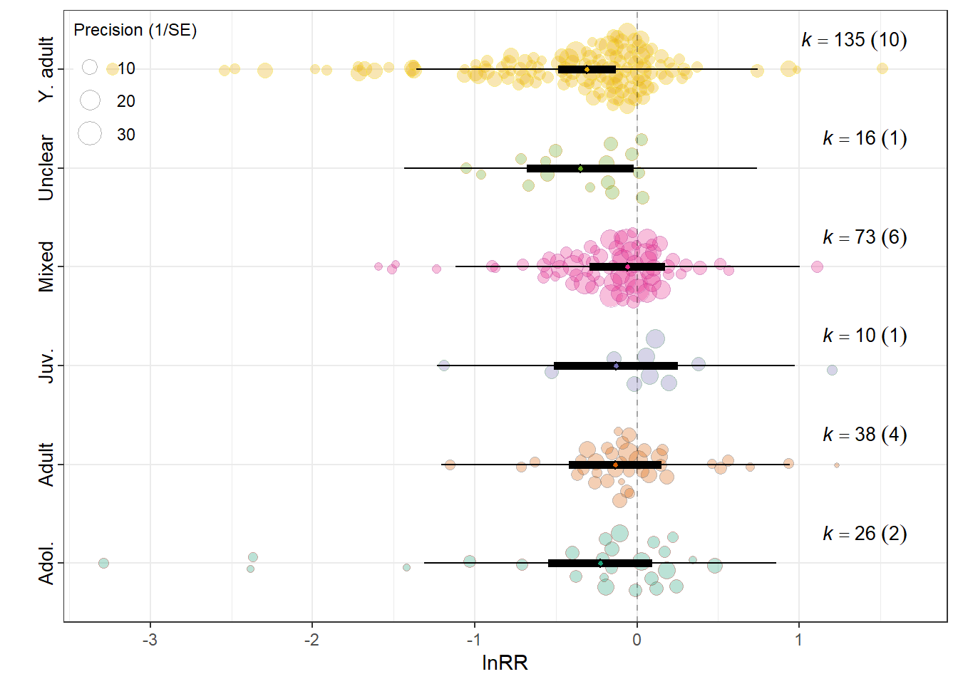
tuk_rr
     Simultaneous Tests for General Linear Hypotheses

Multiple Comparisons of Means: Tukey Contrasts


Fit: metafor::rma.mv(yi = dat[[yi]], V = V, mods = mods_formula, data = dat,
    random = list(~1 | Study_ID, ~1 | ES_ID, ~1 | Strain), method = "REML",
    test = "t", sparse = TRUE)

Linear Hypotheses:
            Estimate Std. Error z value Pr(>|z|)
2 - 1 == 0  0.093666   0.186134   0.503   0.6148
3 - 1 == 0  0.096523   0.208702   0.462   0.6437
4 - 1 == 0  0.167255   0.197336   0.848   0.3967
5 - 1 == 0 -0.122164   0.220161  -0.555   0.5790
6 - 1 == 0 -0.081458   0.166351  -0.490   0.6244
3 - 2 == 0  0.002857   0.206027   0.014   0.9889
4 - 2 == 0  0.073588   0.180845   0.407   0.6841
5 - 2 == 0 -0.215830   0.209449  -1.030   0.3028
6 - 2 == 0 -0.175125   0.152363  -1.149   0.2504
4 - 3 == 0  0.070731   0.223106   0.317   0.7512
5 - 3 == 0 -0.218687   0.241529  -0.905   0.3652
6 - 3 == 0 -0.177982   0.193208  -0.921   0.3569
5 - 4 == 0 -0.289418   0.201759  -1.434   0.1514
6 - 4 == 0 -0.248713   0.143526  -1.733   0.0831 .
6 - 5 == 0  0.040705   0.148271   0.275   0.7837
---
Signif. codes:  0 '***' 0.001 '**' 0.01 '*' 0.05 '.' 0.1 ' ' 1
(Adjusted p values reported -- none method)
lnVR
summary(res_vr$model)
Multivariate Meta-Analysis Model (k = 222; method: REML)

   logLik   Deviance        AIC        BIC       AICc
-339.3525   678.7050   696.7050   727.0825   697.5788

Variance Components:

            estim    sqrt  nlvls  fixed    factor
sigma^2.1  0.0263  0.1621     16     no  Study_ID
sigma^2.2  1.2491  1.1176    222     no     ES_ID
sigma^2.3  0.0000  0.0000      6     no    Strain

Test for Residual Heterogeneity:
QE(df = 216) = 4359.9557, p-val < .0001

Test of Moderators (coefficients 1:6):
F(df1 = 6, df2 = 216) = 1.1160, p-val = 0.3539

Model Results:

                               estimate      se     tval   df    pval    ci.lb
Lifestage_exposureAdolescent     0.7391  0.3236   2.2844  216  0.0233   0.1014
Lifestage_exposureAdult         -0.0508  0.2667  -0.1903  216  0.8492  -0.5764
Lifestage_exposureJuvenile       0.0347  0.5057   0.0685  216  0.9454  -0.9621
Lifestage_exposureMixed         -0.1120  0.2389  -0.4687  216  0.6398  -0.5829
Lifestage_exposureUnclear        0.1922  0.3773   0.5094  216  0.6110  -0.5515
Lifestage_exposureYoung adult    0.1715  0.1561   1.0988  216  0.2731  -0.1361
                                ci.ub
Lifestage_exposureAdolescent   1.3768  *
Lifestage_exposureAdult        0.4749
Lifestage_exposureJuvenile     1.0315
Lifestage_exposureMixed        0.3589
Lifestage_exposureUnclear      0.9359
Lifestage_exposureYoung adult  0.4791

---
Signif. codes: 0 '***' 0.001 '**' 0.01 '*' 0.05 '.' 0.1 ' ' 1res_vr$r2 R2_marginal R2_conditional
0.0388 0.0586 res_vr$plot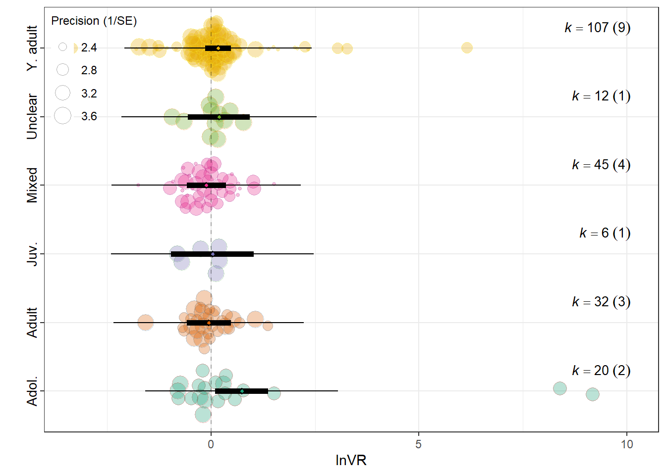
tuk_vr
     Simultaneous Tests for General Linear Hypotheses

Multiple Comparisons of Means: Tukey Contrasts


Fit: metafor::rma.mv(yi = dat[[yi]], V = V, mods = mods_formula, data = dat,
    random = list(~1 | Study_ID, ~1 | ES_ID, ~1 | Strain), method = "REML",
    test = "t", sparse = TRUE)

Linear Hypotheses:
           Estimate Std. Error z value Pr(>|z|)
2 - 1 == 0 -0.78987    0.40549  -1.948   0.0514 .
3 - 1 == 0 -0.70446    0.56920  -1.238   0.2159
4 - 1 == 0 -0.85110    0.40220  -2.116   0.0343 *
5 - 1 == 0 -0.54692    0.49456  -1.106   0.2688
6 - 1 == 0 -0.56763    0.35356  -1.605   0.1084
3 - 2 == 0  0.08541    0.54910   0.156   0.8764
4 - 2 == 0 -0.06122    0.35804  -0.171   0.8642
5 - 2 == 0  0.24296    0.46018   0.528   0.5975
6 - 2 == 0  0.22225    0.30441   0.730   0.4653
4 - 3 == 0 -0.14663    0.55932  -0.262   0.7932
5 - 3 == 0  0.15754    0.62662   0.251   0.8015
6 - 3 == 0  0.13683    0.52068   0.263   0.7927
5 - 4 == 0  0.30418    0.44658   0.681   0.4958
6 - 4 == 0  0.28347    0.28538   0.993   0.3206
6 - 5 == 0 -0.02071    0.37038  -0.056   0.9554
---
Signif. codes:  0 '***' 0.001 '**' 0.01 '*' 0.05 '.' 0.1 ' ' 1
(Adjusted p values reported -- none method)
lnCVR
summary(res_cvr$model)
Multivariate Meta-Analysis Model (k = 222; method: REML)

   logLik   Deviance        AIC        BIC       AICc
-275.4287   550.8573   568.8573   599.2348   569.7311

Variance Components:

            estim    sqrt  nlvls  fixed    factor
sigma^2.1  0.0914  0.3023     16     no  Study_ID
sigma^2.2  0.5881  0.7669    222     no     ES_ID
sigma^2.3  0.0000  0.0000      6     no    Strain

Test for Residual Heterogeneity:
QE(df = 216) = 1529.9807, p-val < .0001

Test of Moderators (coefficients 1:6):
F(df1 = 6, df2 = 216) = 0.8899, p-val = 0.5031

Model Results:

                               estimate      se     tval   df    pval    ci.lb
Lifestage_exposureAdolescent     0.2796  0.3072   0.9103  216  0.3637  -0.3258
Lifestage_exposureAdult         -0.1264  0.2565  -0.4929  216  0.6226  -0.6319
Lifestage_exposureJuvenile      -0.0182  0.3922  -0.0464  216  0.9631  -0.7913
Lifestage_exposureMixed         -0.2921  0.2504  -1.1668  216  0.2446  -0.7856
Lifestage_exposureUnclear       -0.1622  0.3034  -0.5346  216  0.5935  -0.7601
Lifestage_exposureYoung adult    0.1846  0.1625   1.1359  216  0.2573  -0.1357
                                ci.ub
Lifestage_exposureAdolescent   0.8851
Lifestage_exposureAdult        0.3791
Lifestage_exposureJuvenile     0.7549
Lifestage_exposureMixed        0.2014
Lifestage_exposureUnclear      0.4358
Lifestage_exposureYoung adult  0.5048

---
Signif. codes: 0 '***' 0.001 '**' 0.01 '*' 0.05 '.' 0.1 ' ' 1res_cvr$r2 R2_marginal R2_conditional
0.0607 0.1871 res_cvr$plot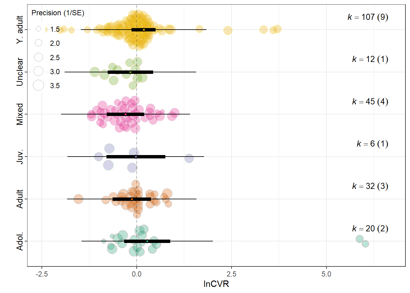
tuk_cvr
     Simultaneous Tests for General Linear Hypotheses

Multiple Comparisons of Means: Tukey Contrasts


Fit: metafor::rma.mv(yi = dat[[yi]], V = V, mods = mods_formula, data = dat,
    random = list(~1 | Study_ID, ~1 | ES_ID, ~1 | Strain), method = "REML",
    test = "t", sparse = TRUE)

Linear Hypotheses:
           Estimate Std. Error z value Pr(>|z|)
2 - 1 == 0 -0.40605    0.35824  -1.133    0.257
3 - 1 == 0 -0.29783    0.43007  -0.693    0.489
4 - 1 == 0 -0.57177    0.39630  -1.443    0.149
5 - 1 == 0 -0.44183    0.41766  -1.058    0.290
6 - 1 == 0 -0.09509    0.32661  -0.291    0.771
3 - 2 == 0  0.10822    0.41552   0.260    0.795
4 - 2 == 0 -0.16572    0.35841  -0.462    0.644
5 - 2 == 0 -0.03579    0.38591  -0.093    0.926
6 - 2 == 0  0.31096    0.28585   1.088    0.277
4 - 3 == 0 -0.27394    0.46532  -0.589    0.556
5 - 3 == 0 -0.14400    0.47772  -0.301    0.763
6 - 3 == 0  0.20274    0.39930   0.508    0.612
5 - 4 == 0  0.12994    0.39335   0.330    0.741
6 - 4 == 0  0.47668    0.29847   1.597    0.110
6 - 5 == 0  0.34674    0.27131   1.278    0.201
(Adjusted p values reported -- none method)
Control conditions
MOD  <- "Control_conditions"
MODS <- "~ `Control_conditions`"

f_rr  <- filter_low_k_single(db_rr,  VCV_rr,  MOD, min_k = 5)
f_vr  <- filter_low_k_single(db_vr,  VCV_vr,  MOD, min_k = 5)
f_cvr <- filter_low_k_single(db_cvr, VCV_cvr, MOD, min_k = 5)

res_rr  <- fit_unimod(f_rr$data,  f_rr$V,  "lnRR",  MODS, MOD, expression(lnRR))
res_vr  <- fit_unimod(f_vr$data,  f_vr$V,  "lnVR",  MODS, MOD, expression(lnVR))
res_cvr <- fit_unimod(f_cvr$data, f_cvr$V, "lnCVR", MODS, MOD, expression(lnCVR))
lnRR
summary(res_rr$model)
Multivariate Meta-Analysis Model (k = 298; method: REML)

   logLik   Deviance        AIC        BIC       AICc
-239.1884   478.3768   488.3768   506.8286   488.5837

Variance Components:

            estim    sqrt  nlvls  fixed    factor
sigma^2.1  0.0454  0.2131     20     no  Study_ID
sigma^2.2  0.2260  0.4754    298     no     ES_ID
sigma^2.3  0.0000  0.0001      6     no    Strain

Test for Residual Heterogeneity:
QE(df = 296) = 5396.0343, p-val < .0001

Test of Moderators (coefficient 2):
F(df1 = 1, df2 = 296) = 6.5356, p-val = 0.0111

Model Results:

                               estimate      se     tval   df    pval    ci.lb
intrcpt                         -0.1871  0.0650  -2.8775  296  0.0043  -0.3151
Control_conditionsWhite noise   -0.2618  0.1024  -2.5565  296  0.0111  -0.4634
                                 ci.ub
intrcpt                        -0.0591  **
Control_conditionsWhite noise  -0.0603   *

---
Signif. codes: 0 '***' 0.001 '**' 0.01 '*' 0.05 '.' 0.1 ' ' 1res_rr$r2 R2_marginal R2_conditional
0.0315 0.1936 res_rr$plot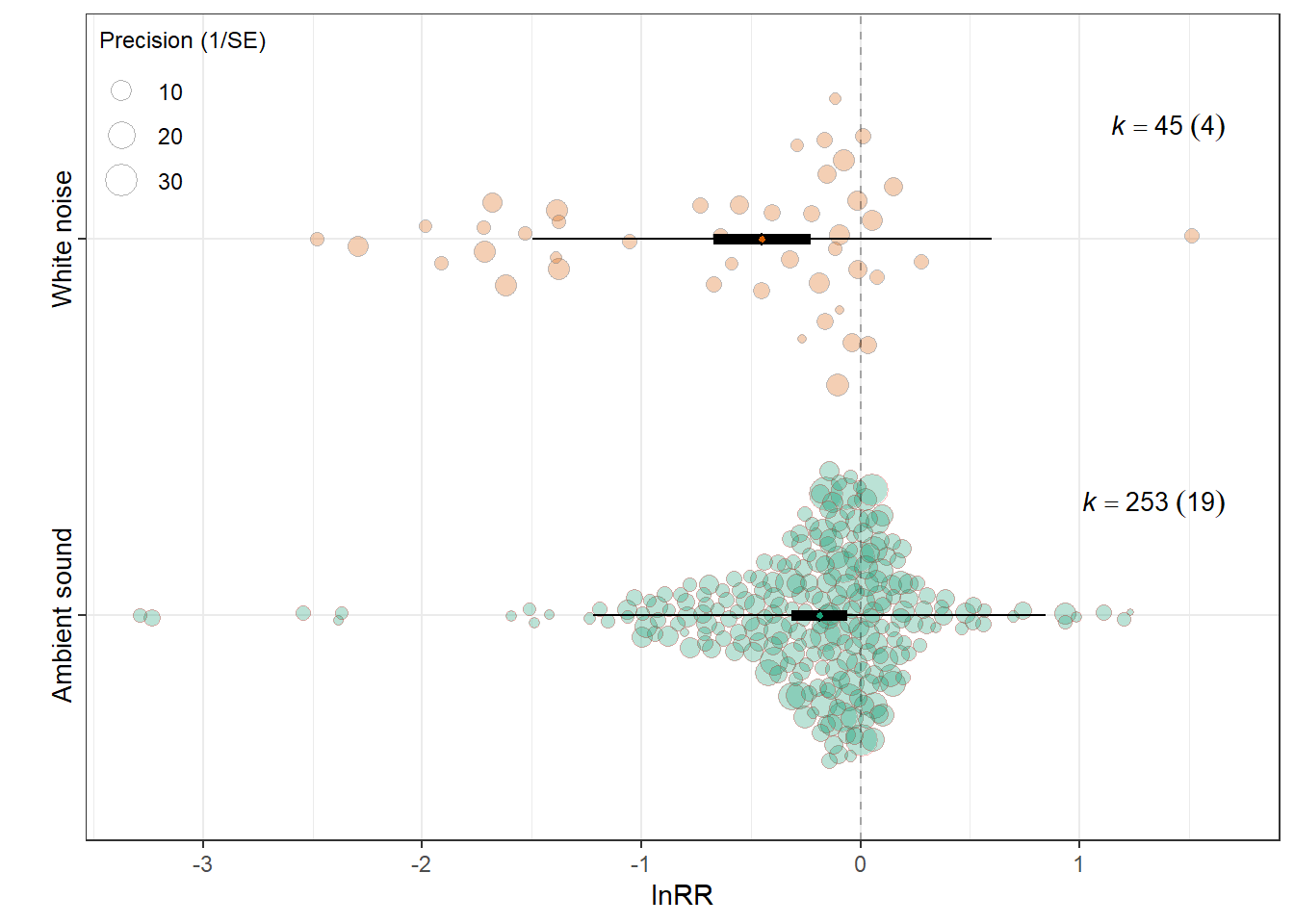
lnVR
summary(res_vr$model)
Multivariate Meta-Analysis Model (k = 222; method: REML)

   logLik   Deviance        AIC        BIC       AICc
-346.6305   693.2609   703.2609   720.2291   703.5413

Variance Components:

            estim    sqrt  nlvls  fixed    factor
sigma^2.1  0.0857  0.2927     16     no  Study_ID
sigma^2.2  1.2273  1.1078    222     no     ES_ID
sigma^2.3  0.0000  0.0001      6     no    Strain

Test for Residual Heterogeneity:
QE(df = 220) = 4380.6933, p-val < .0001

Test of Moderators (coefficient 2):
F(df1 = 1, df2 = 220) = 0.3657, p-val = 0.5460

Model Results:

                               estimate      se     tval   df    pval    ci.lb
intrcpt                          0.1497  0.1311   1.1415  220  0.2549  -0.1087
Control_conditionsWhite noise   -0.1533  0.2535  -0.6047  220  0.5460  -0.6530
                                ci.ub
intrcpt                        0.4081
Control_conditionsWhite noise  0.3463

---
Signif. codes: 0 '***' 0.001 '**' 0.01 '*' 0.05 '.' 0.1 ' ' 1res_vr$r2 R2_marginal R2_conditional
0.0023 0.0674 res_vr$plot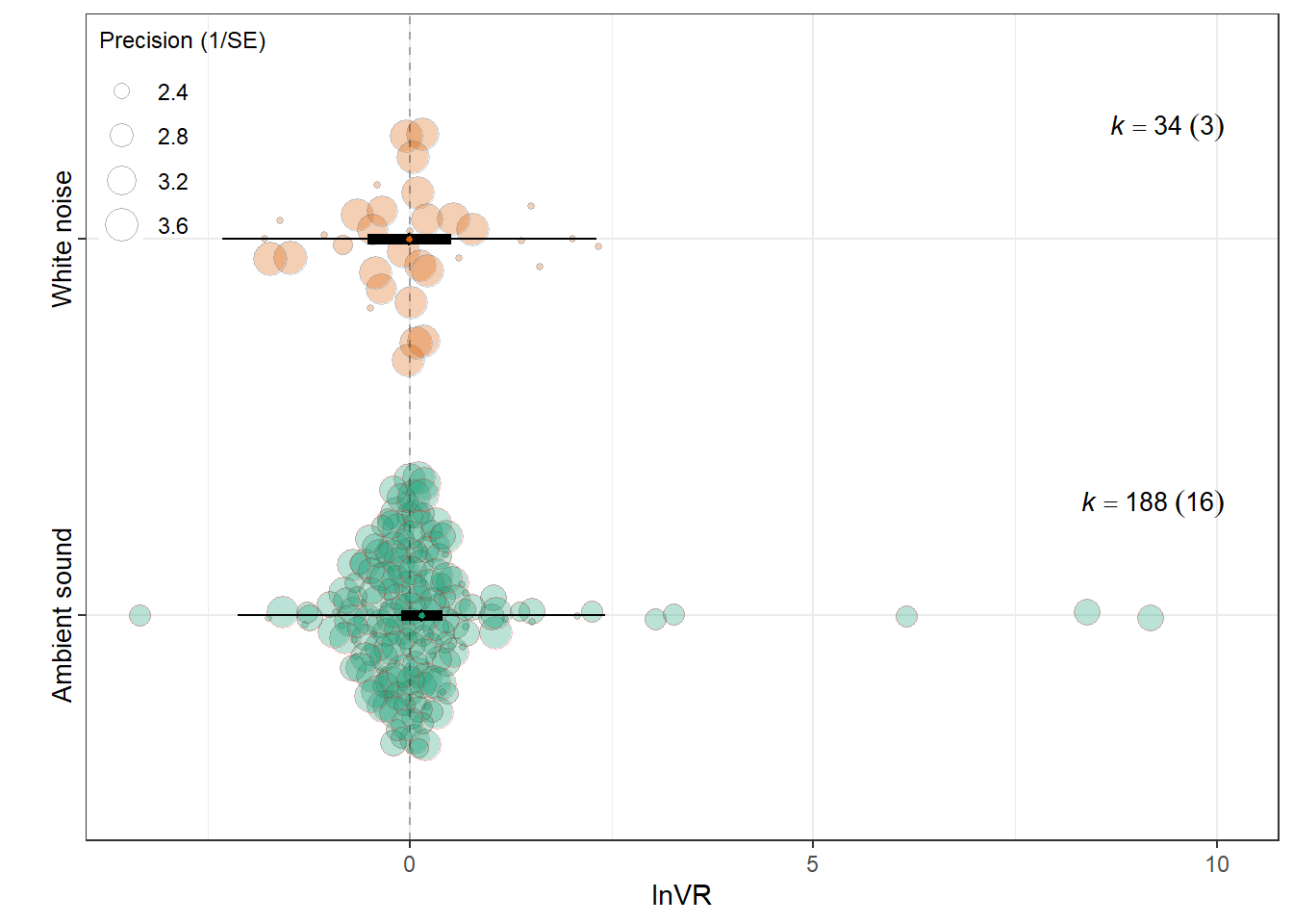
lnCVR
summary(res_cvr$model)
Multivariate Meta-Analysis Model (k = 222; method: REML)

   logLik   Deviance        AIC        BIC       AICc
-281.7941   563.5883   573.5883   590.5564   573.8687

Variance Components:

            estim    sqrt  nlvls  fixed    factor
sigma^2.1  0.0789  0.2808     16     no  Study_ID
sigma^2.2  0.5915  0.7691    222     no     ES_ID
sigma^2.3  0.0000  0.0000      6     no    Strain

Test for Residual Heterogeneity:
QE(df = 220) = 1585.5877, p-val < .0001

Test of Moderators (coefficient 2):
F(df1 = 1, df2 = 220) = 1.7612, p-val = 0.1859

Model Results:

                               estimate      se     tval   df    pval    ci.lb
intrcpt                          0.0380  0.1192   0.3187  220  0.7503  -0.1969
Control_conditionsWhite noise   -0.2540  0.1914  -1.3271  220  0.1859  -0.6313
                                ci.ub
intrcpt                        0.2729
Control_conditionsWhite noise  0.1232

---
Signif. codes: 0 '***' 0.001 '**' 0.01 '*' 0.05 '.' 0.1 ' ' 1res_cvr$r2 R2_marginal R2_conditional
0.0124 0.1286 res_cvr$plot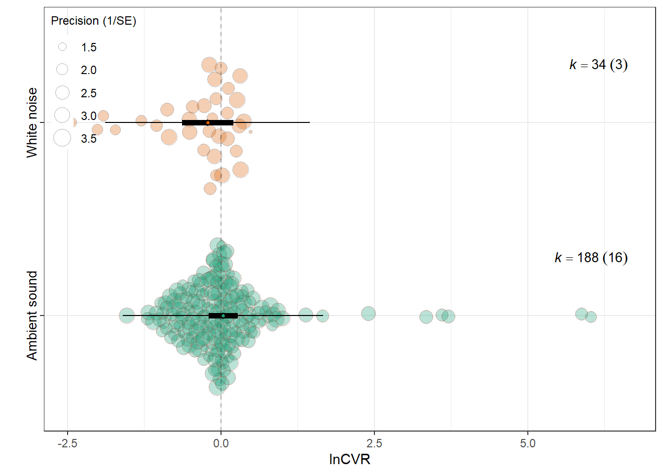
Relative timing
MOD  <- "Relative_timing"
MODS <- "~ Relative_timing -1"


# 1) Filter each effect-size dataset (and subset the VCV accordingly)
f_rr  <- filter_low_k_single(db_rr,  VCV_rr,  MOD, min_k = 5)
f_vr  <- filter_low_k_single(db_vr,  VCV_vr,  MOD, min_k = 5)
f_cvr <- filter_low_k_single(db_cvr, VCV_cvr, MOD, min_k = 5)


# 2) Fit the three unimoderator models (same moderator, different yi/vi)
res_rr  <- fit_unimod(f_rr$data,  f_rr$V,  "lnRR",  MODS, MOD, expression(lnRR))
res_vr  <- fit_unimod(f_vr$data,  f_vr$V,  "lnVR",  MODS, MOD, expression(lnVR))
res_cvr <- fit_unimod(f_cvr$data, f_cvr$V, "lnCVR", MODS, MOD, expression(lnCVR))


# 3) Tukey contrasts (use the filtered data + matched VCV for each dataset)

tuk_rr  <- maybe_tukey(dat = f_rr$data,  V = f_rr$V,  yi = "lnRR",  moderator = MOD)
tuk_vr  <- maybe_tukey(dat = f_vr$data,  V = f_vr$V,  yi = "lnVR",  moderator = MOD)
tuk_cvr <- maybe_tukey(dat = f_cvr$data, V = f_cvr$V, yi = "lnCVR", moderator = MOD)
lnRR
summary(res_rr$model)
Multivariate Meta-Analysis Model (k = 298; method: REML)

   logLik   Deviance        AIC        BIC       AICc
-238.8518   477.7036   489.7036   511.8254   489.9953

Variance Components:

            estim    sqrt  nlvls  fixed    factor
sigma^2.1  0.0495  0.2225     20     no  Study_ID
sigma^2.2  0.2274  0.4768    298     no     ES_ID
sigma^2.3  0.0000  0.0000      6     no    Strain

Test for Residual Heterogeneity:
QE(df = 295) = 5723.3737, p-val < .0001

Test of Moderators (coefficients 1:3):
F(df1 = 3, df2 = 295) = 5.1666, p-val = 0.0017

Model Results:

                           estimate      se     tval   df    pval    ci.lb
Relative_timingBefore       -0.2276  0.0721  -3.1590  295  0.0017  -0.3695
Relative_timingBoth         -0.1965  0.1394  -1.4096  295  0.1597  -0.4707
Relative_timingConcurrent    0.3328  0.2469   1.3475  295  0.1788  -0.1532
                             ci.ub
Relative_timingBefore      -0.0858  **
Relative_timingBoth         0.0778
Relative_timingConcurrent   0.8188

---
Signif. codes: 0 '***' 0.001 '**' 0.01 '*' 0.05 '.' 0.1 ' ' 1res_rr$r2 R2_marginal R2_conditional
0.0220 0.1969 res_rr$plot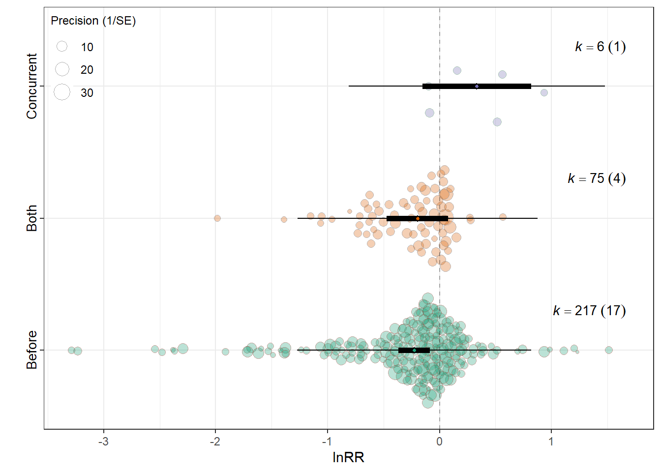
tuk_rr
     Simultaneous Tests for General Linear Hypotheses

Multiple Comparisons of Means: Tukey Contrasts


Fit: metafor::rma.mv(yi = dat[[yi]], V = V, mods = mods_formula, data = dat,
    random = list(~1 | Study_ID, ~1 | ES_ID, ~1 | Strain), method = "REML",
    test = "t", sparse = TRUE)

Linear Hypotheses:
           Estimate Std. Error z value Pr(>|z|)
2 - 1 == 0  0.03119    0.15099   0.207   0.8364
3 - 1 == 0  0.56041    0.24810   2.259   0.0239 *
3 - 2 == 0  0.52922    0.25511   2.074   0.0380 *
---
Signif. codes:  0 '***' 0.001 '**' 0.01 '*' 0.05 '.' 0.1 ' ' 1
(Adjusted p values reported -- none method)
lnVR
summary(res_vr$model)
Multivariate Meta-Analysis Model (k = 222; method: REML)

   logLik   Deviance        AIC        BIC       AICc
-345.0522   690.1044   702.1044   722.4389   702.5006

Variance Components:

            estim    sqrt  nlvls  fixed    factor
sigma^2.1  0.0962  0.3102     16     no  Study_ID
sigma^2.2  1.2301  1.1091    222     no     ES_ID
sigma^2.3  0.0000  0.0001      6     no    Strain

Test for Residual Heterogeneity:
QE(df = 219) = 4389.4876, p-val < .0001

Test of Moderators (coefficients 1:3):
F(df1 = 3, df2 = 219) = 0.4882, p-val = 0.6908

Model Results:

                           estimate      se     tval   df    pval    ci.lb
Relative_timingBefore        0.1733  0.1445   1.1996  219  0.2316  -0.1114
Relative_timingBoth         -0.0209  0.2902  -0.0721  219  0.9426  -0.5928
Relative_timingConcurrent    0.0074  0.5409   0.0136  219  0.9891  -1.0587
                            ci.ub
Relative_timingBefore      0.4581
Relative_timingBoth        0.5509
Relative_timingConcurrent  1.0735

---
Signif. codes: 0 '***' 0.001 '**' 0.01 '*' 0.05 '.' 0.1 ' ' 1res_vr$r2 R2_marginal R2_conditional
0.0055 0.0776 res_vr$plot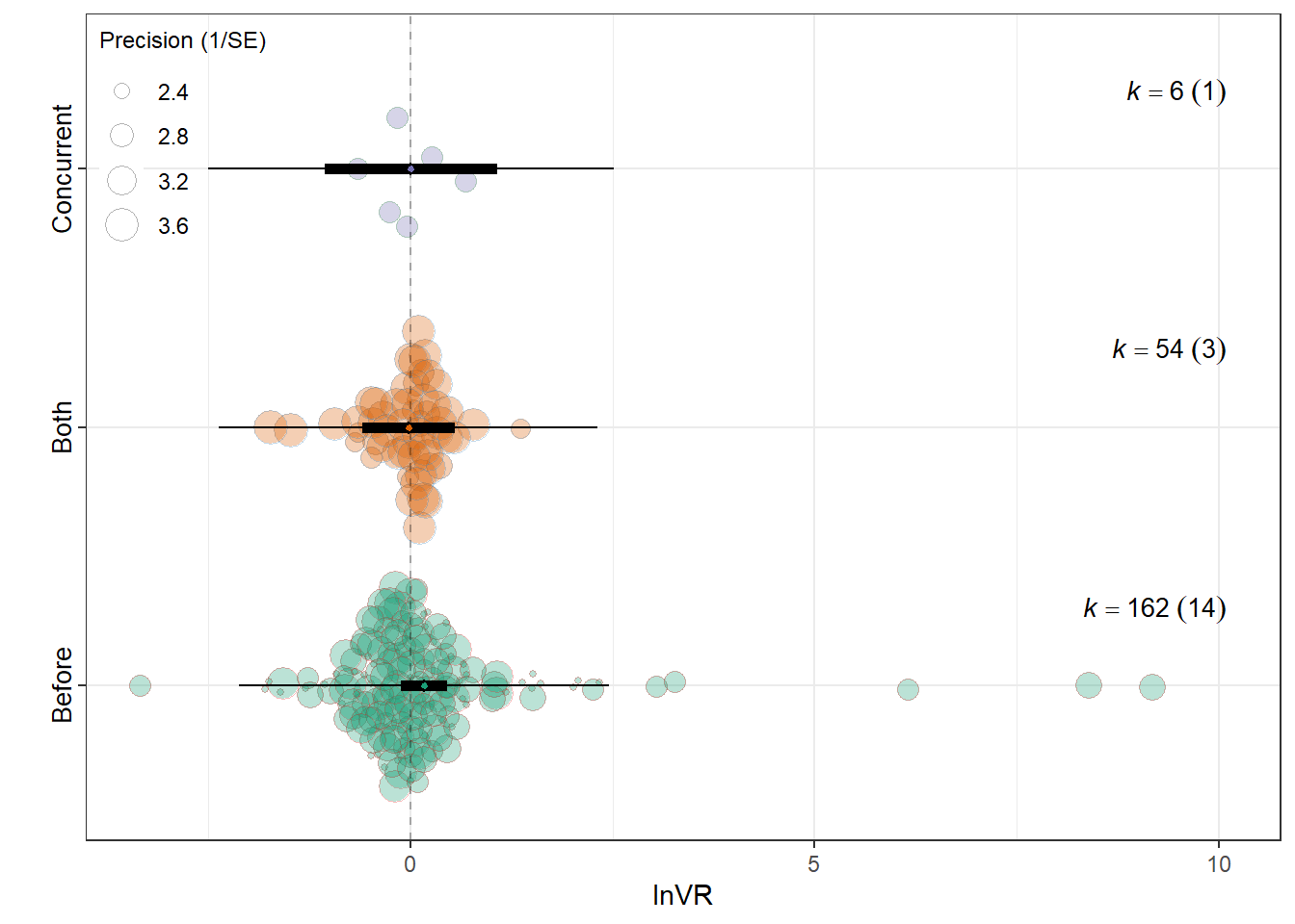
tuk_vr
     Simultaneous Tests for General Linear Hypotheses

Multiple Comparisons of Means: Tukey Contrasts


Fit: metafor::rma.mv(yi = dat[[yi]], V = V, mods = mods_formula, data = dat,
    random = list(~1 | Study_ID, ~1 | ES_ID, ~1 | Strain), method = "REML",
    test = "t", sparse = TRUE)

Linear Hypotheses:
           Estimate Std. Error z value Pr(>|z|)
2 - 1 == 0 -0.19425    0.31647  -0.614    0.539
3 - 1 == 0 -0.16596    0.54716  -0.303    0.762
3 - 2 == 0  0.02829    0.56931   0.050    0.960
(Adjusted p values reported -- none method)
lnCVR
summary(res_cvr$model)
Multivariate Meta-Analysis Model (k = 222; method: REML)

   logLik   Deviance        AIC        BIC       AICc
-281.1298   562.2596   574.2596   594.5940   574.6558

Variance Components:

            estim    sqrt  nlvls  fixed    factor
sigma^2.1  0.1051  0.3241     16     no  Study_ID
sigma^2.2  0.5934  0.7703    222     no     ES_ID
sigma^2.3  0.0000  0.0000      6     no    Strain

Test for Residual Heterogeneity:
QE(df = 219) = 1587.2641, p-val < .0001

Test of Moderators (coefficients 1:3):
F(df1 = 3, df2 = 219) = 0.0805, p-val = 0.9706

Model Results:

                           estimate      se     tval   df    pval    ci.lb
Relative_timingBefore        0.0414  0.1351   0.3062  219  0.7598  -0.2248
Relative_timingBoth         -0.0876  0.2642  -0.3316  219  0.7405  -0.6082
Relative_timingConcurrent   -0.0583  0.4153  -0.1405  219  0.8884  -0.8768
                            ci.ub
Relative_timingBefore      0.3075
Relative_timingBoth        0.4330
Relative_timingConcurrent  0.7601

---
Signif. codes: 0 '***' 0.001 '**' 0.01 '*' 0.05 '.' 0.1 ' ' 1res_cvr$r2 R2_marginal R2_conditional
0.0045 0.1543 res_cvr$plot
tuk_cvr
     Simultaneous Tests for General Linear Hypotheses

Multiple Comparisons of Means: Tukey Contrasts


Fit: metafor::rma.mv(yi = dat[[yi]], V = V, mods = mods_formula, data = dat,
    random = list(~1 | Study_ID, ~1 | ES_ID, ~1 | Strain), method = "REML",
    test = "t", sparse = TRUE)

Linear Hypotheses:
           Estimate Std. Error z value Pr(>|z|)
2 - 1 == 0 -0.12894    0.28206  -0.457    0.648
3 - 1 == 0 -0.09969    0.41646  -0.239    0.811
3 - 2 == 0  0.02925    0.43058   0.068    0.946
(Adjusted p values reported -- none method)
Music genre
MOD  <- "Meta_genre"
MODS <- "~ Meta_genre -1"


genre_labels <- c(
  "Mixed"  = "Mixed",
  "Popular Contemporary Music"       = "Contemporary",
  "Traditional Music / Folk / World"    = "World",
  "Western Art Music / Orchestral" = "Orchestral"
)


# 1) Filter each effect-size dataset (and subset the VCV accordingly)
f_rr  <- filter_low_k_single(db_rr,  VCV_rr,  MOD, min_k = 5)
f_vr  <- filter_low_k_single(db_vr,  VCV_vr,  MOD, min_k = 5)
f_cvr <- filter_low_k_single(db_cvr, VCV_cvr, MOD, min_k = 5)


# 2) Fit the three unimoderator models (same moderator, different yi/vi)
res_rr  <- fit_unimod(f_rr$data,  f_rr$V,  "lnRR",  MODS, MOD, expression(lnRR))
res_vr  <- fit_unimod(f_vr$data,  f_vr$V,  "lnVR",  MODS, MOD, expression(lnVR))
res_cvr <- fit_unimod(f_cvr$data, f_cvr$V, "lnCVR", MODS, MOD, expression(lnCVR))


# 2b) Relabel x-axis in the orchard plots (so EPM/OFT/etc. show)
res_rr$plot  <- res_rr$plot  + scale_x_discrete(labels = genre_labels)
res_vr$plot  <- res_vr$plot  + scale_x_discrete(labels = genre_labels)
res_cvr$plot <- res_cvr$plot + scale_x_discrete(labels = genre_labels)


# 3) Tukey contrasts (use the filtered data + matched VCV for each dataset)

tuk_rr  <- maybe_tukey(dat = f_rr$data,  V = f_rr$V,  yi = "lnRR",  moderator = MOD)
tuk_vr  <- maybe_tukey(dat = f_vr$data,  V = f_vr$V,  yi = "lnVR",  moderator = MOD)
tuk_cvr <- maybe_tukey(dat = f_cvr$data, V = f_cvr$V, yi = "lnCVR", moderator = MOD)
lnRR
summary(res_rr$model)
Multivariate Meta-Analysis Model (k = 298; method: REML)

   logLik   Deviance        AIC        BIC       AICc
-239.2750   478.5500   492.5500   518.3351   492.9416

Variance Components:

            estim    sqrt  nlvls  fixed    factor
sigma^2.1  0.0497  0.2230     20     no  Study_ID
sigma^2.2  0.2304  0.4800    298     no     ES_ID
sigma^2.3  0.0000  0.0000      6     no    Strain

Test for Residual Heterogeneity:
QE(df = 294) = 5718.2060, p-val < .0001

Test of Moderators (coefficients 1:4):
F(df1 = 4, df2 = 294) = 3.2258, p-val = 0.0130

Model Results:

                                            estimate      se     tval   df
Meta_genreMixed                              -0.2143  0.1467  -1.4605  294
Meta_genrePopular Contemporary Music         -0.1015  0.1917  -0.5297  294
Meta_genreTraditional Music / Folk / World   -0.5983  0.2594  -2.3068  294
Meta_genreWestern Art Music / Orchestral     -0.1902  0.0766  -2.4812  294
                                              pval    ci.lb    ci.ub
Meta_genreMixed                             0.1452  -0.5030   0.0745
Meta_genrePopular Contemporary Music        0.5968  -0.4787   0.2757
Meta_genreTraditional Music / Folk / World  0.0218  -1.1088  -0.0878  *
Meta_genreWestern Art Music / Orchestral    0.0137  -0.3410  -0.0393  *

---
Signif. codes: 0 '***' 0.001 '**' 0.01 '*' 0.05 '.' 0.1 ' ' 1res_rr$r2 R2_marginal R2_conditional
0.0232 0.1966 res_rr$plot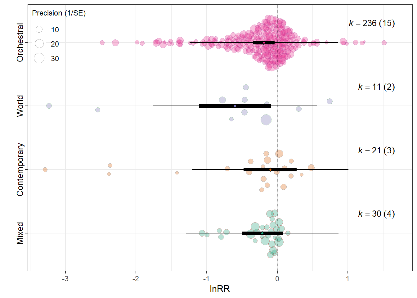
tuk_rr
     Simultaneous Tests for General Linear Hypotheses

Multiple Comparisons of Means: Tukey Contrasts


Fit: metafor::rma.mv(yi = dat[[yi]], V = V, mods = mods_formula, data = dat,
    random = list(~1 | Study_ID, ~1 | ES_ID, ~1 | Strain), method = "REML",
    test = "t", sparse = TRUE)

Linear Hypotheses:
           Estimate Std. Error z value Pr(>|z|)
2 - 1 == 0  0.11277    0.22999   0.490    0.624
3 - 1 == 0 -0.38403    0.29750  -1.291    0.197
4 - 1 == 0  0.02413    0.16005   0.151    0.880
3 - 2 == 0 -0.49680    0.31754  -1.565    0.118
4 - 2 == 0 -0.08864    0.19863  -0.446    0.655
4 - 3 == 0  0.40816    0.26934   1.515    0.130
(Adjusted p values reported -- none method)
lnVR
summary(res_vr$model)
Multivariate Meta-Analysis Model (k = 222; method: REML)

   logLik   Deviance        AIC        BIC       AICc
-338.3565   676.7131   690.7131   714.4045   691.2464

Variance Components:

            estim    sqrt  nlvls  fixed    factor
sigma^2.1  0.0000  0.0000     16     no  Study_ID
sigma^2.2  1.2200  1.1045    222     no     ES_ID
sigma^2.3  0.0000  0.0000      6     no    Strain

Test for Residual Heterogeneity:
QE(df = 218) = 4375.2042, p-val < .0001

Test of Moderators (coefficients 1:4):
F(df1 = 4, df2 = 218) = 3.7277, p-val = 0.0059

Model Results:

                                            estimate      se     tval   df
Meta_genreMixed                              -0.0639  0.2850  -0.2243  218
Meta_genrePopular Contemporary Music          0.9563  0.3203   2.9859  218
Meta_genreTraditional Music / Folk / World    1.1263  0.4627   2.4341  218
Meta_genreWestern Art Music / Orchestral     -0.0212  0.1180  -0.1793  218
                                              pval    ci.lb   ci.ub
Meta_genreMixed                             0.8228  -0.6256  0.4978
Meta_genrePopular Contemporary Music        0.0032   0.3251  1.5876  **
Meta_genreTraditional Music / Folk / World  0.0157   0.2143  2.0383   *
Meta_genreWestern Art Music / Orchestral    0.8579  -0.2538  0.2115

---
Signif. codes: 0 '***' 0.001 '**' 0.01 '*' 0.05 '.' 0.1 ' ' 1res_vr$r2 R2_marginal R2_conditional
0.0841 0.0841 res_vr$plot
tuk_vr
     Simultaneous Tests for General Linear Hypotheses

Multiple Comparisons of Means: Tukey Contrasts


Fit: metafor::rma.mv(yi = dat[[yi]], V = V, mods = mods_formula, data = dat,
    random = list(~1 | Study_ID, ~1 | ES_ID, ~1 | Strain), method = "REML",
    test = "t", sparse = TRUE)

Linear Hypotheses:
           Estimate Std. Error z value Pr(>|z|)
2 - 1 == 0  1.02023    0.42497   2.401   0.0164 *
3 - 1 == 0  1.19024    0.54342   2.190   0.0285 *
4 - 1 == 0  0.04276    0.30703   0.139   0.8892
3 - 2 == 0  0.17001    0.56173   0.303   0.7622
4 - 2 == 0 -0.97748    0.33961  -2.878   0.0040 **
4 - 3 == 0 -1.14749    0.47737  -2.404   0.0162 *
---
Signif. codes:  0 '***' 0.001 '**' 0.01 '*' 0.05 '.' 0.1 ' ' 1
(Adjusted p values reported -- none method)
lnCVR
summary(res_cvr$model)
Multivariate Meta-Analysis Model (k = 222; method: REML)

   logLik   Deviance        AIC        BIC       AICc
-273.3294   546.6587   560.6587   584.3502   561.1921

Variance Components:

            estim    sqrt  nlvls  fixed    factor
sigma^2.1  0.0000  0.0000     16     no  Study_ID
sigma^2.2  0.5893  0.7676    222     no     ES_ID
sigma^2.3  0.0000  0.0000      6     no    Strain

Test for Residual Heterogeneity:
QE(df = 218) = 1563.1637, p-val < .0001

Test of Moderators (coefficients 1:4):
F(df1 = 4, df2 = 218) = 3.9471, p-val = 0.0041

Model Results:

                                            estimate      se     tval   df
Meta_genreMixed                              -0.0789  0.2334  -0.3381  218
Meta_genrePopular Contemporary Music          0.4492  0.2853   1.5742  218
Meta_genreTraditional Music / Folk / World    1.3149  0.3865   3.4019  218
Meta_genreWestern Art Music / Orchestral     -0.1322  0.1071  -1.2342  218
                                              pval    ci.lb   ci.ub
Meta_genreMixed                             0.7356  -0.5390  0.3812
Meta_genrePopular Contemporary Music        0.1169  -0.1132  1.0116
Meta_genreTraditional Music / Folk / World  0.0008   0.5531  2.0767  ***
Meta_genreWestern Art Music / Orchestral    0.2185  -0.3433  0.0789

---
Signif. codes: 0 '***' 0.001 '**' 0.01 '*' 0.05 '.' 0.1 ' ' 1res_cvr$r2 R2_marginal R2_conditional
0.1359 0.1359 res_cvr$plot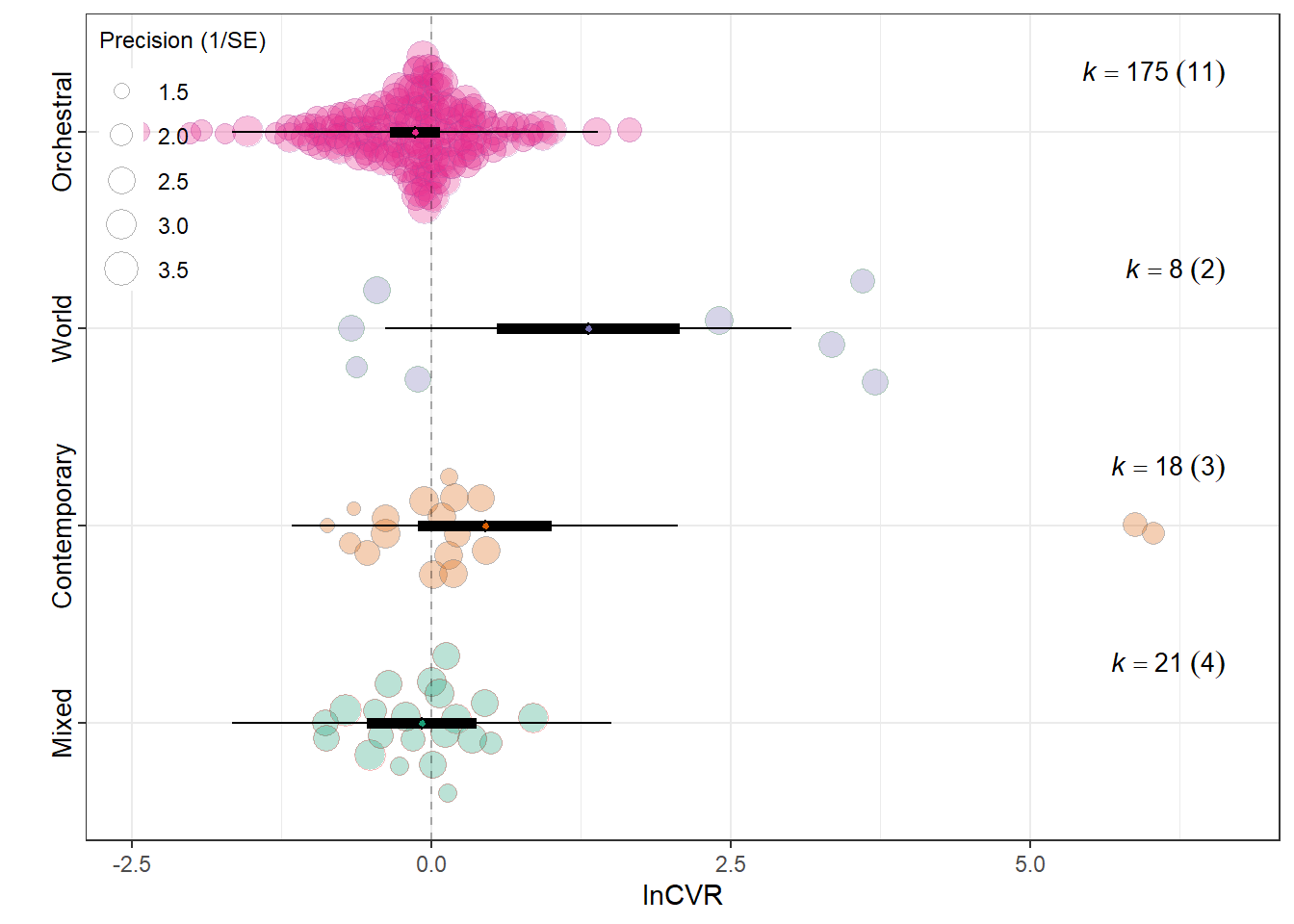
tuk_cvr
     Simultaneous Tests for General Linear Hypotheses

Multiple Comparisons of Means: Tukey Contrasts


Fit: metafor::rma.mv(yi = dat[[yi]], V = V, mods = mods_formula, data = dat,
    random = list(~1 | Study_ID, ~1 | ES_ID, ~1 | Strain), method = "REML",
    test = "t", sparse = TRUE)

Linear Hypotheses:
           Estimate Std. Error z value Pr(>|z|)
2 - 1 == 0  0.52809    0.36032   1.466 0.142754
3 - 1 == 0  1.39383    0.45139   3.088 0.002016 **
4 - 1 == 0 -0.05327    0.25340  -0.210 0.833498
3 - 2 == 0  0.86574    0.47712   1.815 0.069597 .
4 - 2 == 0 -0.58136    0.30018  -1.937 0.052781 .
4 - 3 == 0 -1.44710    0.40050  -3.613 0.000302 ***
---
Signif. codes:  0 '***' 0.001 '**' 0.01 '*' 0.05 '.' 0.1 ' ' 1
(Adjusted p values reported -- none method)
Experimental design
MOD  <- "Experimental_design"
MODS <- "~ Experimental_design -1"


design_labels<-c(
  "Factorial"="Factorial",
  "Posttest-Only Control Group"="Posttest",
  "Repeated Measures"="Repeated"

)


# 1) Filter each effect-size dataset (and subset the VCV accordingly)
f_rr  <- filter_low_k_single(db_rr,  VCV_rr,  MOD, min_k = 5)
f_vr  <- filter_low_k_single(db_vr,  VCV_vr,  MOD, min_k = 5)
f_cvr <- filter_low_k_single(db_cvr, VCV_cvr, MOD, min_k = 5)


# 2) Fit the three unimoderator models (same moderator, different yi/vi)
res_rr  <- fit_unimod(f_rr$data,  f_rr$V,  "lnRR",  MODS, MOD, expression(lnRR))
res_vr  <- fit_unimod(f_vr$data,  f_vr$V,  "lnVR",  MODS, MOD, expression(lnVR))
res_cvr <- fit_unimod(f_cvr$data, f_cvr$V, "lnCVR", MODS, MOD, expression(lnCVR))


# 2b) Relabel x-axis in the orchard plots (so EPM/OFT/etc. show)
res_rr$plot  <- res_rr$plot  + scale_x_discrete(labels = design_labels)
res_vr$plot  <- res_vr$plot  + scale_x_discrete(labels = design_labels)
res_cvr$plot <- res_cvr$plot + scale_x_discrete(labels = design_labels)


# 3) Tukey contrasts (use the filtered data + matched VCV for each dataset)

tuk_rr  <- maybe_tukey(dat = f_rr$data,  V = f_rr$V,  yi = "lnRR",  moderator = MOD)
tuk_vr  <- maybe_tukey(dat = f_vr$data,  V = f_vr$V,  yi = "lnVR",  moderator = MOD)
tuk_cvr <- maybe_tukey(dat = f_cvr$data, V = f_cvr$V, yi = "lnCVR", moderator = MOD)
lnRR
summary(res_rr$model)
Multivariate Meta-Analysis Model (k = 298; method: REML)

   logLik   Deviance        AIC        BIC       AICc
-239.2296   478.4593   490.4593   512.5811   490.7509

Variance Components:

            estim    sqrt  nlvls  fixed    factor
sigma^2.1  0.0442  0.2102     20     no  Study_ID
sigma^2.2  0.2297  0.4793    298     no     ES_ID
sigma^2.3  0.0000  0.0000      6     no    Strain

Test for Residual Heterogeneity:
QE(df = 295) = 5684.0603, p-val < .0001

Test of Moderators (coefficients 1:3):
F(df1 = 3, df2 = 295) = 5.0020, p-val = 0.0021

Model Results:

                                                estimate      se     tval   df
Experimental_designFactorial                     -0.1772  0.0704  -2.5178  295
Experimental_designPosttest-Only Control Group   -0.3808  0.1066  -3.5735  295
Experimental_designRepeated Measures             -0.1624  0.2051  -0.7915  295
                                                  pval    ci.lb    ci.ub
Experimental_designFactorial                    0.0123  -0.3157  -0.0387    *
Experimental_designPosttest-Only Control Group  0.0004  -0.5905  -0.1711  ***
Experimental_designRepeated Measures            0.4293  -0.5660   0.2413

---
Signif. codes: 0 '***' 0.001 '**' 0.01 '*' 0.05 '.' 0.1 ' ' 1res_rr$r2 R2_marginal R2_conditional
0.0224 0.1801 res_rr$plot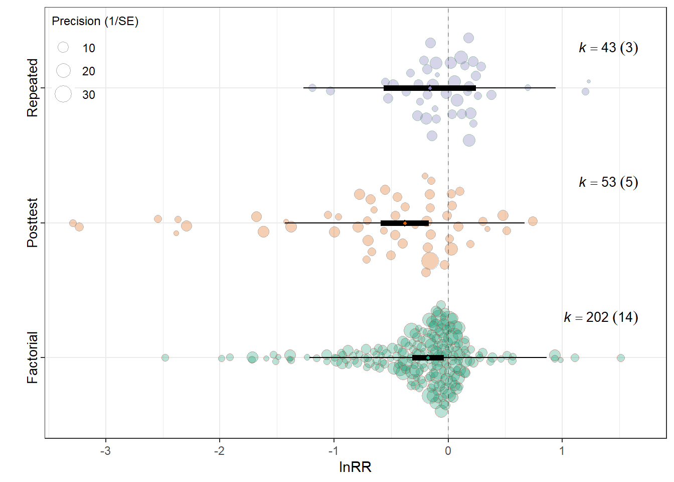
tuk_rr
     Simultaneous Tests for General Linear Hypotheses

Multiple Comparisons of Means: Tukey Contrasts


Fit: metafor::rma.mv(yi = dat[[yi]], V = V, mods = mods_formula, data = dat,
    random = list(~1 | Study_ID, ~1 | ES_ID, ~1 | Strain), method = "REML",
    test = "t", sparse = TRUE)

Linear Hypotheses:
           Estimate Std. Error z value Pr(>|z|)
2 - 1 == 0 -0.20356    0.10332  -1.970   0.0488 *
3 - 1 == 0  0.01485    0.21686   0.068   0.9454
3 - 2 == 0  0.21841    0.23115   0.945   0.3447
---
Signif. codes:  0 '***' 0.001 '**' 0.01 '*' 0.05 '.' 0.1 ' ' 1
(Adjusted p values reported -- none method)
lnVR
summary(res_vr$model)
Multivariate Meta-Analysis Model (k = 222; method: REML)

   logLik   Deviance        AIC        BIC       AICc
-341.4846   682.9693   694.9693   715.3037   695.3655

Variance Components:

            estim    sqrt  nlvls  fixed    factor
sigma^2.1  0.0000  0.0001     16     no  Study_ID
sigma^2.2  1.2318  1.1099    222     no     ES_ID
sigma^2.3  0.0000  0.0000      6     no    Strain

Test for Residual Heterogeneity:
QE(df = 219) = 4376.1207, p-val < .0001

Test of Moderators (coefficients 1:3):
F(df1 = 3, df2 = 219) = 3.6274, p-val = 0.0138

Model Results:

                                                estimate      se     tval   df
Experimental_designFactorial                      0.0225  0.1185   0.1899  219
Experimental_designPosttest-Only Control Group    0.6459  0.2007   3.2188  219
Experimental_designRepeated Measures             -0.2031  0.3078  -0.6598  219
                                                  pval    ci.lb   ci.ub
Experimental_designFactorial                    0.8496  -0.2110  0.2560
Experimental_designPosttest-Only Control Group  0.0015   0.2504  1.0414  **
Experimental_designRepeated Measures            0.5101  -0.8097  0.4035

---
Signif. codes: 0 '***' 0.001 '**' 0.01 '*' 0.05 '.' 0.1 ' ' 1res_vr$r2 R2_marginal R2_conditional
0.056 0.056 res_vr$plot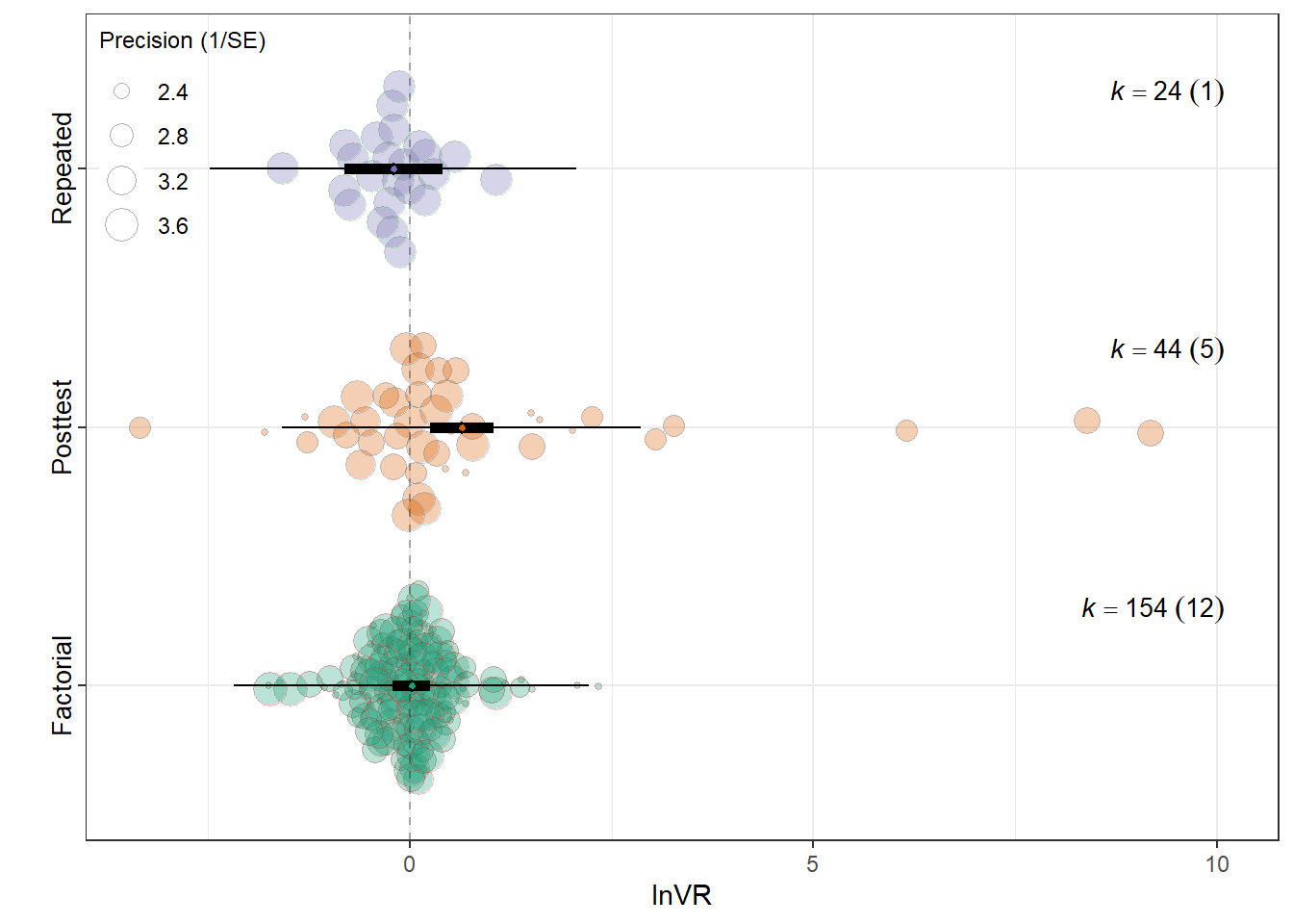
tuk_vr
     Simultaneous Tests for General Linear Hypotheses

Multiple Comparisons of Means: Tukey Contrasts


Fit: metafor::rma.mv(yi = dat[[yi]], V = V, mods = mods_formula, data = dat,
    random = list(~1 | Study_ID, ~1 | ES_ID, ~1 | Strain), method = "REML",
    test = "t", sparse = TRUE)

Linear Hypotheses:
           Estimate Std. Error z value Pr(>|z|)
2 - 1 == 0   0.6234     0.2173   2.869  0.00412 **
3 - 1 == 0  -0.2256     0.3298  -0.684  0.49399
3 - 2 == 0  -0.8490     0.3674  -2.311  0.02085 *
---
Signif. codes:  0 '***' 0.001 '**' 0.01 '*' 0.05 '.' 0.1 ' ' 1
(Adjusted p values reported -- none method)
lnCVR
summary(res_cvr$model)
Multivariate Meta-Analysis Model (k = 222; method: REML)

   logLik   Deviance        AIC        BIC       AICc
-280.1420   560.2840   572.2840   592.6184   572.6802

Variance Components:

            estim    sqrt  nlvls  fixed    factor
sigma^2.1  0.0560  0.2366     16     no  Study_ID
sigma^2.2  0.5990  0.7739    222     no     ES_ID
sigma^2.3  0.0000  0.0000      6     no    Strain

Test for Residual Heterogeneity:
QE(df = 219) = 1585.4977, p-val < .0001

Test of Moderators (coefficients 1:3):
F(df1 = 3, df2 = 219) = 0.7164, p-val = 0.5431

Model Results:

                                                estimate      se     tval   df
Experimental_designFactorial                     -0.0239  0.1243  -0.1926  219
Experimental_designPosttest-Only Control Group    0.2250  0.1831   1.2286  219
Experimental_designRepeated Measures             -0.1655  0.3664  -0.4516  219
                                                  pval    ci.lb   ci.ub
Experimental_designFactorial                    0.8475  -0.2689  0.2210
Experimental_designPosttest-Only Control Group  0.2205  -0.1359  0.5859
Experimental_designRepeated Measures            0.6520  -0.8876  0.5567

---
Signif. codes: 0 '***' 0.001 '**' 0.01 '*' 0.05 '.' 0.1 ' ' 1res_cvr$r2 R2_marginal R2_conditional
0.0200 0.1038 res_cvr$plot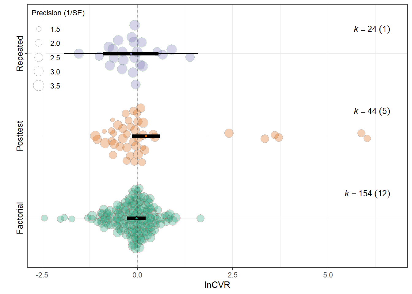
tuk_cvr
     Simultaneous Tests for General Linear Hypotheses

Multiple Comparisons of Means: Tukey Contrasts


Fit: metafor::rma.mv(yi = dat[[yi]], V = V, mods = mods_formula, data = dat,
    random = list(~1 | Study_ID, ~1 | ES_ID, ~1 | Strain), method = "REML",
    test = "t", sparse = TRUE)

Linear Hypotheses:
           Estimate Std. Error z value Pr(>|z|)
2 - 1 == 0   0.2489     0.1821   1.367    0.172
3 - 1 == 0  -0.1415     0.3869  -0.366    0.715
3 - 2 == 0  -0.3904     0.4096  -0.953    0.341
(Adjusted p values reported -- none method)
Sex
MOD  <- "Sex"
MODS <- "~ Sex"

f_rr  <- filter_low_k_single(db_rr,  VCV_rr,  MOD, min_k = 5)
f_vr  <- filter_low_k_single(db_vr,  VCV_vr,  MOD, min_k = 5)
f_cvr <- filter_low_k_single(db_cvr, VCV_cvr, MOD, min_k = 5)

res_rr  <- fit_unimod(f_rr$data,  f_rr$V,  "lnRR",  MODS, MOD, expression(lnRR))
res_vr  <- fit_unimod(f_vr$data,  f_vr$V,  "lnVR",  MODS, MOD, expression(lnVR))
res_cvr <- fit_unimod(f_cvr$data, f_cvr$V, "lnCVR", MODS, MOD, expression(lnCVR))
lnRR
summary(res_rr$model)
Multivariate Meta-Analysis Model (k = 295; method: REML)

   logLik   Deviance        AIC        BIC       AICc
-238.9455   477.8911   487.8911   506.2920   488.1002

Variance Components:

            estim    sqrt  nlvls  fixed    factor
sigma^2.1  0.0420  0.2050     19     no  Study_ID
sigma^2.2  0.2300  0.4796    295     no     ES_ID
sigma^2.3  0.0096  0.0981      6     no    Strain

Test for Residual Heterogeneity:
QE(df = 293) = 5730.3718, p-val < .0001

Test of Moderators (coefficient 2):
F(df1 = 1, df2 = 293) = 2.7371, p-val = 0.0991

Model Results:

         estimate      se     tval   df    pval    ci.lb    ci.ub
intrcpt   -0.3100  0.1015  -3.0543  293  0.0025  -0.5098  -0.1103  **
SexMale    0.1529  0.0924   1.6544  293  0.0991  -0.0290   0.3348   .

---
Signif. codes: 0 '***' 0.001 '**' 0.01 '*' 0.05 '.' 0.1 ' ' 1res_rr$r2 R2_marginal R2_conditional
0.0194 0.1993 res_rr$plot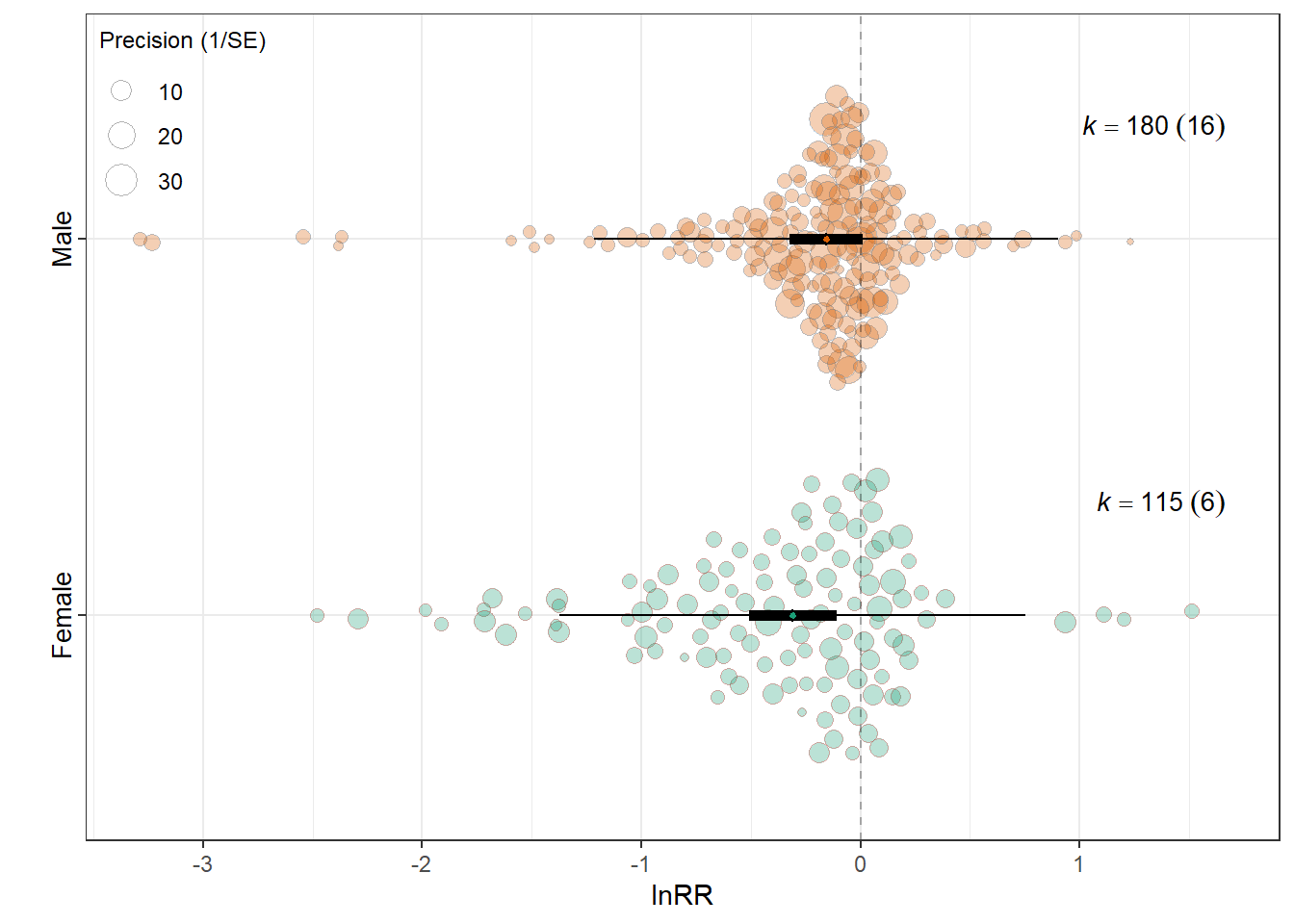
lnVR
summary(res_vr$model)
Multivariate Meta-Analysis Model (k = 219; method: REML)

   logLik   Deviance        AIC        BIC       AICc
-342.8395   685.6790   695.6790   712.5785   695.9634

Variance Components:

            estim    sqrt  nlvls  fixed    factor
sigma^2.1  0.0900  0.3001     15     no  Study_ID
sigma^2.2  1.2406  1.1138    219     no     ES_ID
sigma^2.3  0.0000  0.0001      6     no    Strain

Test for Residual Heterogeneity:
QE(df = 217) = 4383.5230, p-val < .0001

Test of Moderators (coefficient 2):
F(df1 = 1, df2 = 217) = 0.3114, p-val = 0.5774

Model Results:

         estimate      se    tval   df    pval    ci.lb   ci.ub
intrcpt    0.0666  0.2034  0.3275  217  0.7436  -0.3342  0.4675
SexMale    0.1276  0.2287  0.5580  217  0.5774  -0.3232  0.5784

---
Signif. codes: 0 '***' 0.001 '**' 0.01 '*' 0.05 '.' 0.1 ' ' 1res_vr$r2 R2_marginal R2_conditional
0.0030 0.0704 res_vr$plot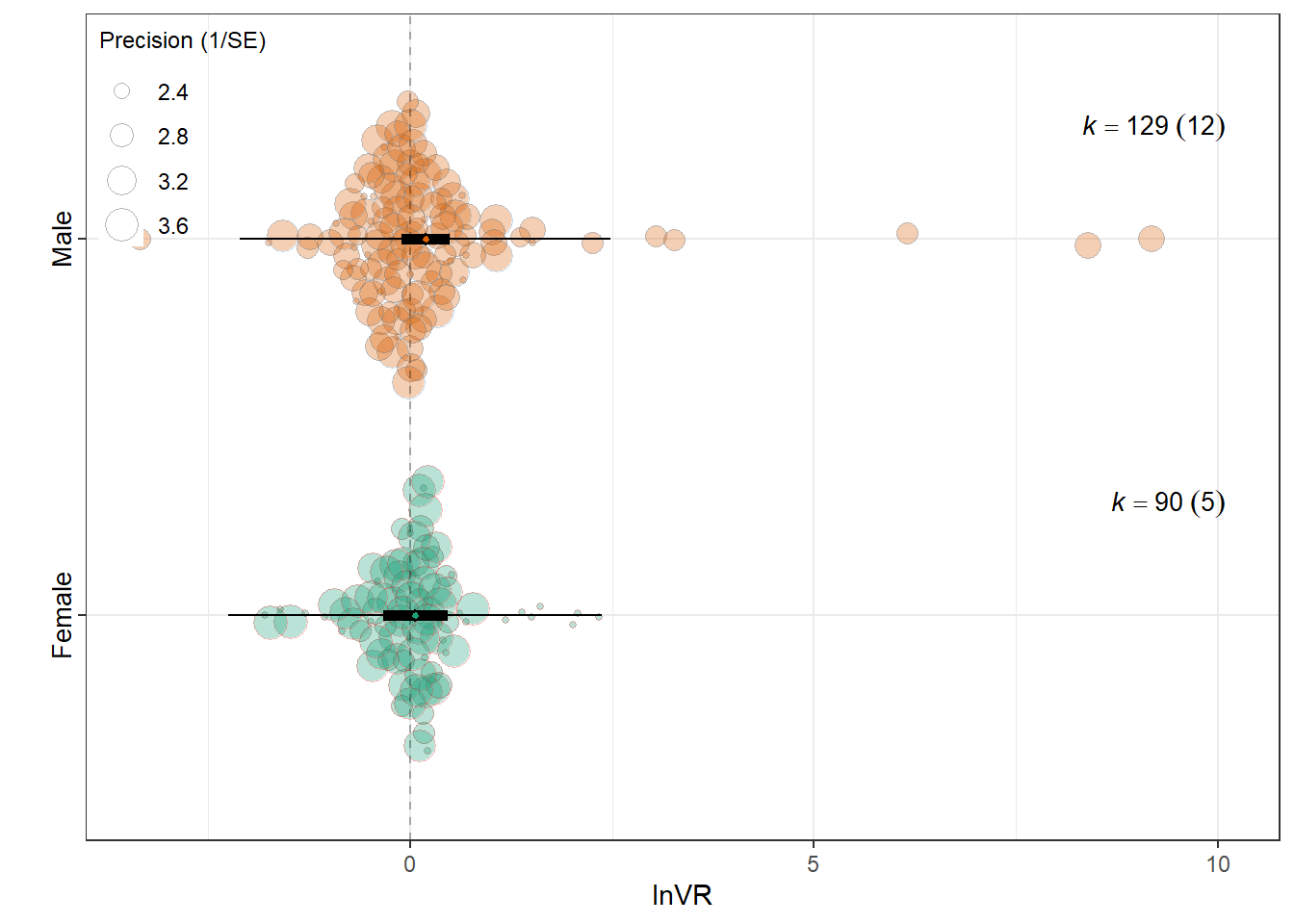
lnCVR
summary(res_cvr$model)
Multivariate Meta-Analysis Model (k = 219; method: REML)

   logLik   Deviance        AIC        BIC       AICc
-278.1954   556.3907   566.3907   583.2902   566.6751

Variance Components:

            estim    sqrt  nlvls  fixed    factor
sigma^2.1  0.0692  0.2630     15     no  Study_ID
sigma^2.2  0.5972  0.7728    219     no     ES_ID
sigma^2.3  0.0000  0.0000      6     no    Strain

Test for Residual Heterogeneity:
QE(df = 217) = 1572.7582, p-val < .0001

Test of Moderators (coefficient 2):
F(df1 = 1, df2 = 217) = 2.0491, p-val = 0.1537

Model Results:

         estimate      se     tval   df    pval    ci.lb   ci.ub
intrcpt   -0.1386  0.1715  -0.8083  217  0.4198  -0.4766  0.1994
SexMale    0.2616  0.1827   1.4315  217  0.1537  -0.0986  0.6217

---
Signif. codes: 0 '***' 0.001 '**' 0.01 '*' 0.05 '.' 0.1 ' ' 1res_cvr$r2 R2_marginal R2_conditional
0.0244 0.1256 res_cvr$plot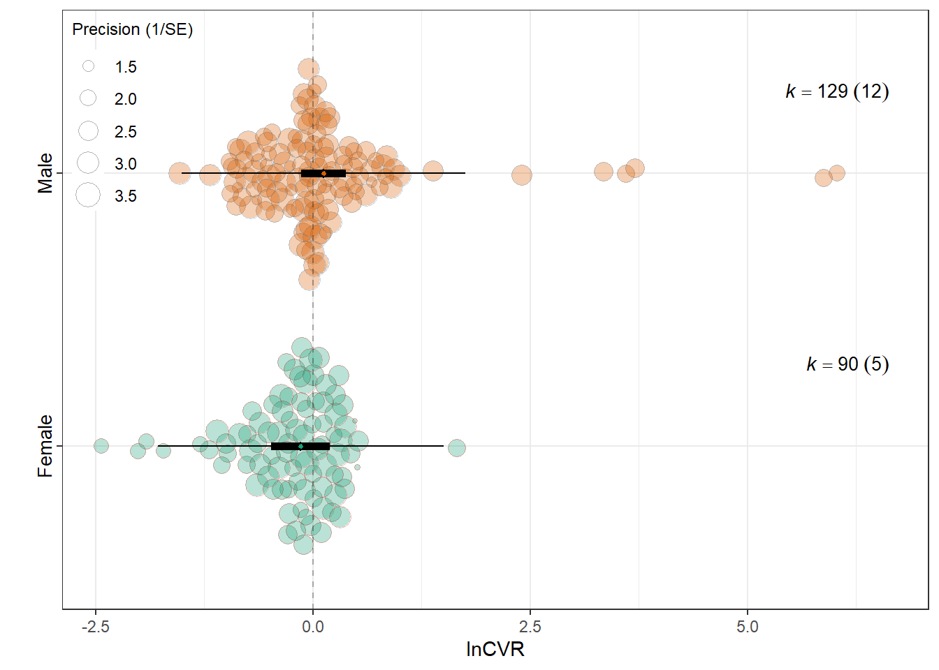
Exposure duration
Music_exposure_duration
MOD  <- "Music_exposure_duration"
MODS <- "~ Music_exposure_duration -1"


# 1) Filter each effect-size dataset (and subset the VCV accordingly)
f_rr  <- filter_low_k_single(db_rr,  VCV_rr,  MOD, min_k = 5)
f_vr  <- filter_low_k_single(db_vr,  VCV_vr,  MOD, min_k = 5)
f_cvr <- filter_low_k_single(db_cvr, VCV_cvr, MOD, min_k = 5)


# 2) Fit the three unimoderator models (same moderator, different yi/vi)
res_rr  <- fit_unimod(f_rr$data,  f_rr$V,  "lnRR",  MODS, MOD, expression(lnRR))
res_vr  <- fit_unimod(f_vr$data,  f_vr$V,  "lnVR",  MODS, MOD, expression(lnVR))
res_cvr <- fit_unimod(f_cvr$data, f_cvr$V, "lnCVR", MODS, MOD, expression(lnCVR))


# 3) Tukey contrasts (use the filtered data + matched VCV for each dataset)

tuk_rr  <- maybe_tukey(dat = f_rr$data,  V = f_rr$V,  yi = "lnRR",  moderator = MOD)
tuk_vr  <- maybe_tukey(dat = f_vr$data,  V = f_vr$V,  yi = "lnVR",  moderator = MOD)
tuk_cvr <- maybe_tukey(dat = f_cvr$data, V = f_cvr$V, yi = "lnCVR", moderator = MOD)
lnRR
summary(res_rr$model)
Multivariate Meta-Analysis Model (k = 297; method: REML)

   logLik   Deviance        AIC        BIC       AICc
-239.5997   479.1994   491.1994   513.3009   491.4921

Variance Components:

            estim    sqrt  nlvls  fixed    factor
sigma^2.1  0.0512  0.2263     20     no  Study_ID
sigma^2.2  0.2319  0.4816    297     no     ES_ID
sigma^2.3  0.0000  0.0000      6     no    Strain

Test for Residual Heterogeneity:
QE(df = 294) = 5777.2420, p-val < .0001

Test of Moderators (coefficients 1:3):
F(df1 = 3, df2 = 294) = 3.8341, p-val = 0.0102

Model Results:

                               estimate      se     tval   df    pval    ci.lb
Music_exposure_durationAcute    -0.2660  0.1118  -2.3798  294  0.0180  -0.4860
Music_exposure_durationMedium   -0.0642  0.1396  -0.4599  294  0.6459  -0.3389
Music_exposure_durationShort    -0.2495  0.1052  -2.3722  294  0.0183  -0.4566
                                 ci.ub
Music_exposure_durationAcute   -0.0460  *
Music_exposure_durationMedium   0.2105
Music_exposure_durationShort   -0.0425  *

---
Signif. codes: 0 '***' 0.001 '**' 0.01 '*' 0.05 '.' 0.1 ' ' 1res_rr$r2 R2_marginal R2_conditional
0.0216 0.1986 res_rr$plot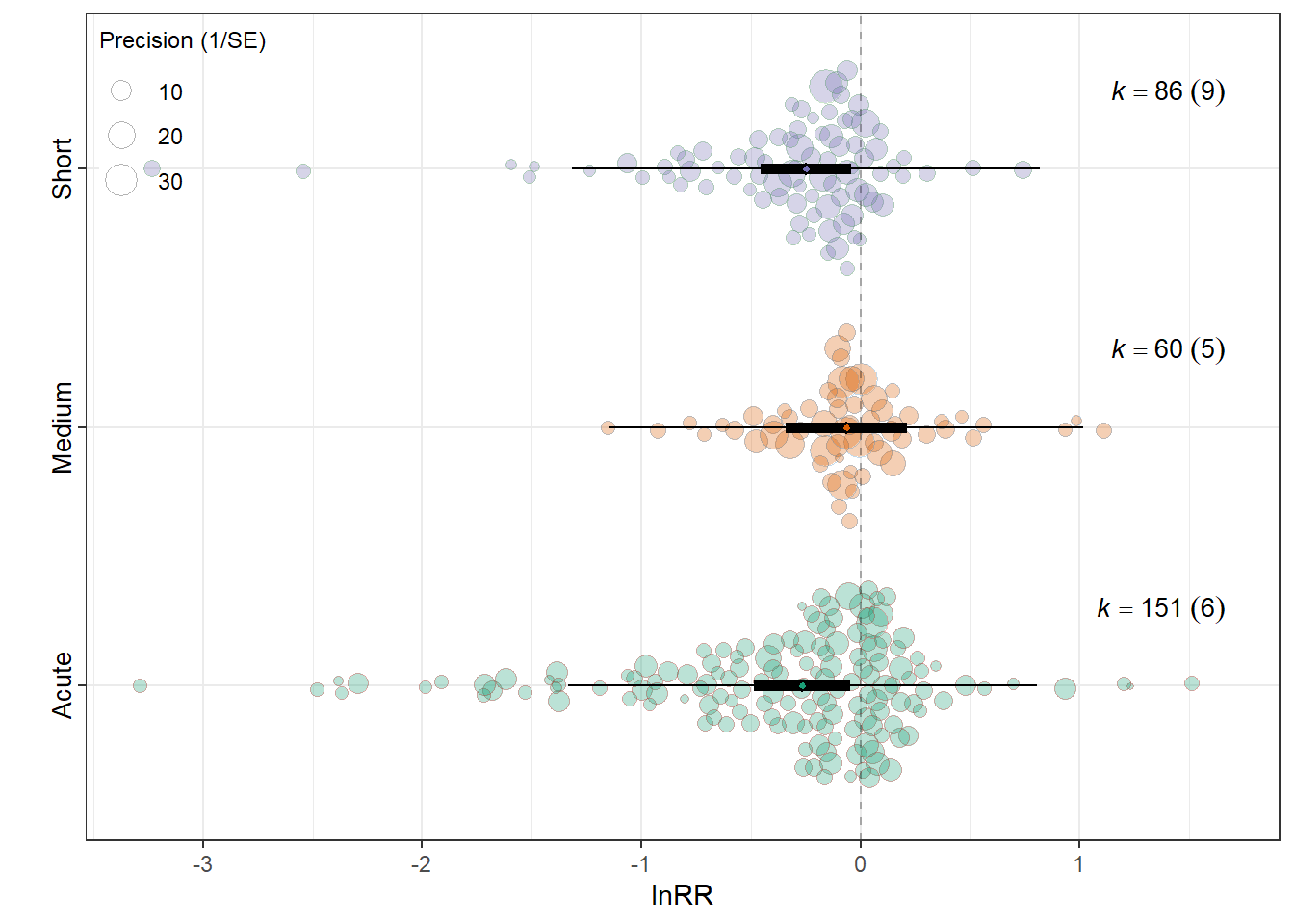
tuk_rr
     Simultaneous Tests for General Linear Hypotheses

Multiple Comparisons of Means: Tukey Contrasts


Fit: metafor::rma.mv(yi = dat[[yi]], V = V, mods = mods_formula, data = dat,
    random = list(~1 | Study_ID, ~1 | ES_ID, ~1 | Strain), method = "REML",
    test = "t", sparse = TRUE)

Linear Hypotheses:
           Estimate Std. Error z value Pr(>|z|)
2 - 1 == 0  0.20184    0.17884   1.129    0.259
3 - 1 == 0  0.01649    0.15350   0.107    0.914
3 - 2 == 0 -0.18535    0.17479  -1.060    0.289
(Adjusted p values reported -- none method)
lnVR
summary(res_vr$model)
Multivariate Meta-Analysis Model (k = 222; method: REML)

   logLik   Deviance        AIC        BIC       AICc
-344.5642   689.1285   701.1285   721.4629   701.5247

Variance Components:

            estim    sqrt  nlvls  fixed    factor
sigma^2.1  0.1181  0.3437     16     no  Study_ID
sigma^2.2  1.2224  1.1056    222     no     ES_ID
sigma^2.3  0.0000  0.0001      6     no    Strain

Test for Residual Heterogeneity:
QE(df = 219) = 4390.2022, p-val < .0001

Test of Moderators (coefficients 1:3):
F(df1 = 3, df2 = 219) = 0.5542, p-val = 0.6458

Model Results:

                               estimate      se    tval   df    pval    ci.lb
Music_exposure_durationAcute     0.2718  0.2202  1.2345  219  0.2183  -0.1621
Music_exposure_durationMedium    0.0052  0.2628  0.0198  219  0.9843  -0.5127
Music_exposure_durationShort     0.0873  0.2348  0.3717  219  0.7105  -0.3754
                                ci.ub
Music_exposure_durationAcute   0.7057
Music_exposure_durationMedium  0.5231
Music_exposure_durationShort   0.5499

---
Signif. codes: 0 '***' 0.001 '**' 0.01 '*' 0.05 '.' 0.1 ' ' 1res_vr$r2 R2_marginal R2_conditional
0.0101 0.0973 res_vr$plot
tuk_vr
     Simultaneous Tests for General Linear Hypotheses

Multiple Comparisons of Means: Tukey Contrasts


Fit: metafor::rma.mv(yi = dat[[yi]], V = V, mods = mods_formula, data = dat,
    random = list(~1 | Study_ID, ~1 | ES_ID, ~1 | Strain), method = "REML",
    test = "t", sparse = TRUE)

Linear Hypotheses:
           Estimate Std. Error z value Pr(>|z|)
2 - 1 == 0 -0.26659    0.34281  -0.778    0.437
3 - 1 == 0 -0.18452    0.32184  -0.573    0.566
3 - 2 == 0  0.08207    0.35236   0.233    0.816
(Adjusted p values reported -- none method)
lnCVR
summary(res_cvr$model)
Multivariate Meta-Analysis Model (k = 222; method: REML)

   logLik   Deviance        AIC        BIC       AICc
-280.5247   561.0493   573.0493   593.3838   573.4456

Variance Components:

            estim    sqrt  nlvls  fixed    factor
sigma^2.1  0.1365  0.3695     16     no  Study_ID
sigma^2.2  0.5889  0.7674    222     no     ES_ID
sigma^2.3  0.0000  0.0000      6     no    Strain

Test for Residual Heterogeneity:
QE(df = 219) = 1588.0953, p-val < .0001

Test of Moderators (coefficients 1:3):
F(df1 = 3, df2 = 219) = 0.0367, p-val = 0.9906

Model Results:

                               estimate      se     tval   df    pval    ci.lb
Music_exposure_durationAcute     0.0200  0.2204   0.0907  219  0.9278  -0.4143
Music_exposure_durationMedium   -0.0405  0.2568  -0.1579  219  0.8747  -0.5466
Music_exposure_durationShort     0.0610  0.2200   0.2771  219  0.7820  -0.3726
                                ci.ub
Music_exposure_durationAcute   0.4543
Music_exposure_durationMedium  0.4655
Music_exposure_durationShort   0.4945

---
Signif. codes: 0 '***' 0.001 '**' 0.01 '*' 0.05 '.' 0.1 ' ' 1res_cvr$r2 R2_marginal R2_conditional
0.0018 0.1897 res_cvr$plot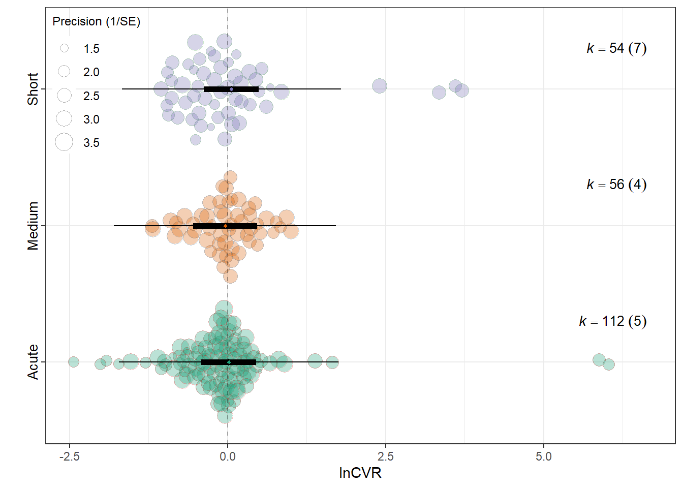
tuk_cvr
     Simultaneous Tests for General Linear Hypotheses

Multiple Comparisons of Means: Tukey Contrasts


Fit: metafor::rma.mv(yi = dat[[yi]], V = V, mods = mods_formula, data = dat,
    random = list(~1 | Study_ID, ~1 | ES_ID, ~1 | Strain), method = "REML",
    test = "t", sparse = TRUE)

Linear Hypotheses:
           Estimate Std. Error z value Pr(>|z|)
2 - 1 == 0 -0.06054    0.33837  -0.179    0.858
3 - 1 == 0  0.04097    0.31138   0.132    0.895
3 - 2 == 0  0.10151    0.33811   0.300    0.764
(Adjusted p values reported -- none method)
Experimental procedure
MOD  <- "Experimental_procedures"
MODS <- "~ Experimental_procedures"

f_rr  <- filter_low_k_single(db_rr,  VCV_rr,  MOD, min_k = 5)
f_vr  <- filter_low_k_single(db_vr,  VCV_vr,  MOD, min_k = 5)
f_cvr <- filter_low_k_single(db_cvr, VCV_cvr, MOD, min_k = 5)

res_rr  <- fit_unimod(f_rr$data,  f_rr$V,  "lnRR",  MODS, MOD, expression(lnRR))
res_vr  <- fit_unimod(f_vr$data,  f_vr$V,  "lnVR",  MODS, MOD, expression(lnVR))
res_cvr <- fit_unimod(f_cvr$data, f_cvr$V, "lnCVR", MODS, MOD, expression(lnCVR))
lnRR
summary(res_rr$model)
Multivariate Meta-Analysis Model (k = 298; method: REML)

   logLik   Deviance        AIC        BIC       AICc
-241.9324   483.8649   493.8649   512.3167   494.0718

Variance Components:

            estim    sqrt  nlvls  fixed    factor
sigma^2.1  0.0546  0.2337     20     no  Study_ID
sigma^2.2  0.2291  0.4786    298     no     ES_ID
sigma^2.3  0.0000  0.0000      6     no    Strain

Test for Residual Heterogeneity:
QE(df = 296) = 5737.2572, p-val < .0001

Test of Moderators (coefficient 2):
F(df1 = 1, df2 = 296) = 0.6644, p-val = 0.4157

Model Results:

                             estimate      se     tval   df    pval    ci.lb
intrcpt                       -0.2227  0.0696  -3.1977  296  0.0015  -0.3597
Experimental_proceduresSham    0.0892  0.1094   0.8151  296  0.4157  -0.1262
                               ci.ub
intrcpt                      -0.0856  **
Experimental_proceduresSham   0.3045

---
Signif. codes: 0 '***' 0.001 '**' 0.01 '*' 0.05 '.' 0.1 ' ' 1res_rr$r2 R2_marginal R2_conditional
0.0045 0.1961 res_rr$plot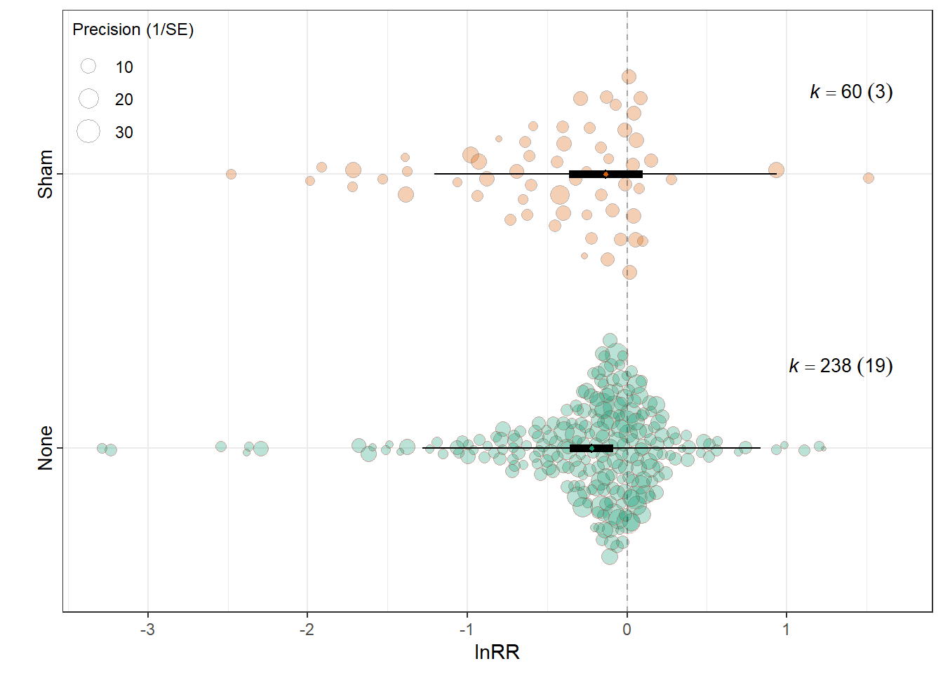
lnVR
summary(res_vr$model)
Multivariate Meta-Analysis Model (k = 222; method: REML)

   logLik   Deviance        AIC        BIC       AICc
-346.5640   693.1281   703.1281   720.0962   703.4085

Variance Components:

            estim    sqrt  nlvls  fixed    factor
sigma^2.1  0.0901  0.3001     16     no  Study_ID
sigma^2.2  1.2265  1.1075    222     no     ES_ID
sigma^2.3  0.0000  0.0001      6     no    Strain

Test for Residual Heterogeneity:
QE(df = 220) = 4386.6575, p-val < .0001

Test of Moderators (coefficient 2):
F(df1 = 1, df2 = 220) = 0.2591, p-val = 0.6112

Model Results:

                             estimate      se     tval   df    pval    ci.lb
intrcpt                        0.1558  0.1362   1.1438  220  0.2539  -0.1126
Experimental_proceduresSham   -0.1239  0.2434  -0.5090  220  0.6112  -0.6036
                              ci.ub
intrcpt                      0.4242
Experimental_proceduresSham  0.3558

---
Signif. codes: 0 '***' 0.001 '**' 0.01 '*' 0.05 '.' 0.1 ' ' 1res_vr$r2 R2_marginal R2_conditional
0.0021 0.0704 res_vr$plot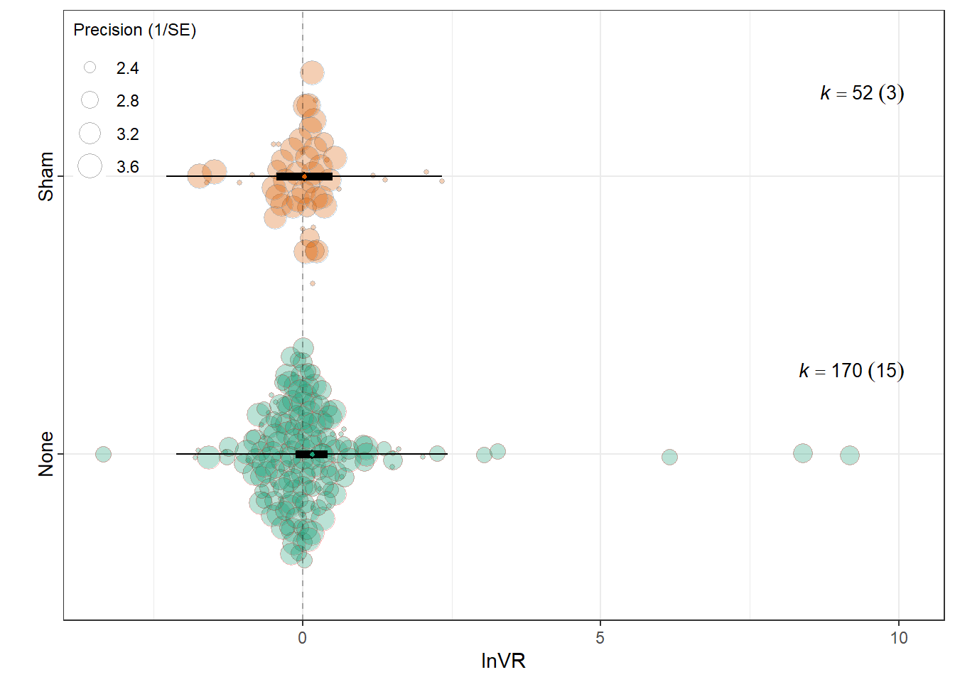
lnCVR
summary(res_cvr$model)
Multivariate Meta-Analysis Model (k = 222; method: REML)

   logLik   Deviance        AIC        BIC       AICc
-282.4682   564.9365   574.9365   591.9046   575.2168

Variance Components:

            estim    sqrt  nlvls  fixed    factor
sigma^2.1  0.0911  0.3019     16     no  Study_ID
sigma^2.2  0.5936  0.7705    222     no     ES_ID
sigma^2.3  0.0000  0.0000      6     no    Strain

Test for Residual Heterogeneity:
QE(df = 220) = 1584.4200, p-val < .0001

Test of Moderators (coefficient 2):
F(df1 = 1, df2 = 220) = 0.0651, p-val = 0.7989

Model Results:

                             estimate      se     tval   df    pval    ci.lb
intrcpt                        0.0246  0.1252   0.1963  220  0.8446  -0.2221
Experimental_proceduresSham   -0.0492  0.1927  -0.2551  220  0.7989  -0.4289
                              ci.ub
intrcpt                      0.2712
Experimental_proceduresSham  0.3306

---
Signif. codes: 0 '***' 0.001 '**' 0.01 '*' 0.05 '.' 0.1 ' ' 1res_cvr$r2 R2_marginal R2_conditional
0.0006 0.1336 res_cvr$plot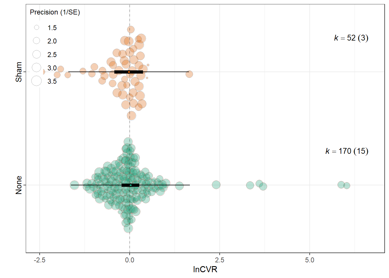
Note
sessionInfo()R version 4.5.2 (2025-10-31 ucrt)
Platform: x86_64-w64-mingw32/x64
Running under: Windows 11 x64 (build 26200)
Matrix products: default
LAPACK version 3.12.1
locale:
[1] LC_COLLATE=English_Guernsey.utf8 LC_CTYPE=English_Guernsey.utf8
[3] LC_MONETARY=English_Guernsey.utf8 LC_NUMERIC=C
[5] LC_TIME=English_Guernsey.utf8
time zone: America/Edmonton
tzcode source: internal
attached base packages:
[1] stats graphics grDevices utils datasets methods base
other attached packages:
[1] multcomp_1.4-29 TH.data_1.1-5 MASS_7.3-65
[4] survival_3.8-6 mvtnorm_1.3-3 orchaRd_2.1.3
[7] metafor_4.8-0 numDeriv_2016.8-1.1 metadat_1.4-0
[10] Matrix_1.7-4 patchwork_1.3.2 lubridate_1.9.4
[13] forcats_1.0.1 stringr_1.6.0 dplyr_1.1.4
[16] purrr_1.2.1 readr_2.1.6 tidyr_1.3.2
[19] tibble_3.3.1 ggplot2_4.0.1 tidyverse_2.0.0
[22] knitr_1.51 here_1.0.2 dtplyr_1.3.2
[25] DT_0.34.0
loaded via a namespace (and not attached):
[1] beeswarm_0.4.0 gtable_0.3.6 xfun_0.56
[4] htmlwidgets_1.6.4 lattice_0.22-7 mathjaxr_2.0-0
[7] tzdb_0.5.0 vctrs_0.7.1 tools_4.5.2
[10] generics_0.1.4 parallel_4.5.2 sandwich_3.1-1
[13] pacman_0.5.1 pkgconfig_2.0.3 data.table_1.18.2.1
[16] RColorBrewer_1.1-3 S7_0.2.1 lifecycle_1.0.5
[19] compiler_4.5.2 farver_2.1.2 codetools_0.2-20
[22] vipor_0.4.7 htmltools_0.5.9 yaml_2.3.12
[25] crayon_1.5.3 pillar_1.11.1 nlme_3.1-168
[28] tidyselect_1.2.1 digest_0.6.39 stringi_1.8.7
[31] labeling_0.4.3 splines_4.5.2 latex2exp_0.9.8
[34] rprojroot_2.1.1 fastmap_1.2.0 grid_4.5.2
[37] cli_3.6.5 magrittr_2.0.4 withr_3.0.2
[40] scales_1.4.0 bit64_4.6.0-1 ggbeeswarm_0.7.3
[43] estimability_1.5.1 timechange_0.3.0 rmarkdown_2.30
[46] emmeans_2.0.1 bit_4.6.0 otel_0.2.0
[49] zoo_1.8-15 hms_1.1.4 coda_0.19-4.1
[52] evaluate_1.0.5 rlang_1.1.7 xtable_1.8-4
[55] glue_1.8.0 rstudioapi_0.18.0 vroom_1.7.0
[58] jsonlite_2.0.0 R6_2.6.1