filter_low_k <- function(dat, V, moderator, min_k = 5) {
  moderator <- rlang::ensym(moderator)
  k_counts <- dat %>%
    dplyr::count(!!moderator, name = "k_es")
  keep_levels <- k_counts %>% dplyr::filter(k_es >= min_k) %>% dplyr::pull(!!moderator)
  dat_f <- dat %>% dplyr::filter((!!moderator) %in% keep_levels)
  idx <- which(dat[[rlang::as_string(moderator)]] %in% keep_levels)
  V_f <- V[idx, idx]
  list(data = dat_f, V = V_f, keep = keep_levels, k = k_counts)
}Code for figures
Note
Variable definitions:
| Variable Name | Definition |
|---|---|
ES_ID |
Unique row identifier for each \(\text{lnRR}\) effect size. |
Study_ID |
Identifier for the primary research paper. |
Cohort_ID |
Identifier for specific experimental groups within a study. |
Outcome_type |
The behavioral construct measured. Levels: Anxiety, Depression, both, unclear. |
Lifestage_exposure |
Animal’s developmental stage during music exposure. Levels: Adolescent, Juvenile, Young adult, Adult, Mixed, Unclear. |
Sex |
Sex of the subjects. Levels: Male, Female. |
Strain |
Specific animal strain or species used. |
Meta_genre |
Categorization of the music stimulus. Levels: Western Art Music / Orchestral, Popular Contemporary Music, Traditional Music / Folk / World, Mixed, Unclear. |
Music_exposure_duration |
Total time subjects were exposed to music. Levels: Acute, short, medium, long. |
Experimental_design |
Study’s methodological setup. Levels: Posttest-Only Control Group, Randomized Block, Factorial, Repeated Measures. |
Induced behavior |
Whether the tested behavior was innate or experimentally induced. |
Relative_timing |
When music was administered relative to the behavioral test. Levels: before, concurrent, both, not specified. |
Experimental_procedures |
Identifies non-treatment controls for interventions. Levels: sham, none. |
Control_condition |
Description of the control group condition. Levels: white noise, ambient noise |
Assay_type |
Type of behavioral test used. |
Overall_rob |
Overall risk of bias assessment for each study. Levels: 2 (low), 1 (moderate), 0 (high). |
NoteData Filtering & Matrix Alignment
We exclude moderator levels with fewer than five effect sizes (k < 5) to avoid unstable estimates and misleading contrasts.
lnRR
ma_all <- rma.mv(yi = lnRR,
                  V = VCV,
                  random = list(~1 | Study_ID,
                                ~1 | ES_ID,
                                ~1 | Strain),
                  test = "t",
                  method = "REML",
                  sparse = TRUE,
                  data = db )

overall_lnRR<-orchard_plot(ma_all,
              group = "Study_ID",
              xlab = "lnRR",
              flip=T,trunk.size = 0.3,
              branch.size = 2,alpha = 0.3) +
              scale_x_discrete(labels = c("Overall effect")) +
            scale_colour_brewer(palette = "Paired") +
            scale_fill_brewer(palette = "Dark2")+
                scale_y_continuous(breaks = seq(-4, 2, by = 1),
                                   minor_breaks = seq(-4, 2, by = 0.5 ))
overall_lnRR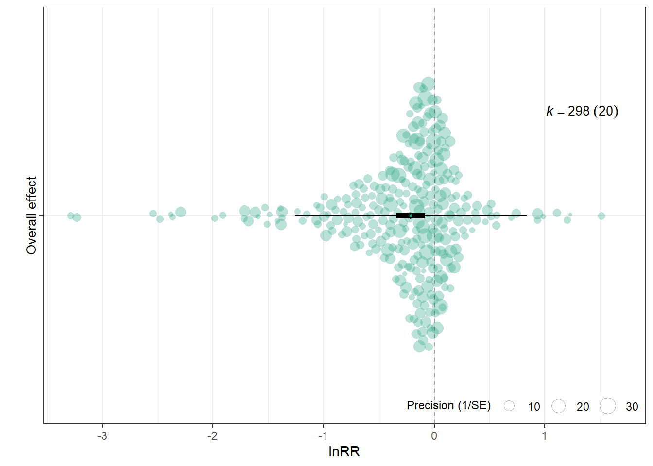
f <- filter_low_k(db, VCV,Outcome_type, min_k = 5)
db_filtered <- f$data
VCV_filtered <- f$V


mOT <- rma.mv(yi = lnRR,
                  V = VCV_filtered,
              mods = ~ Outcome_type,
                  random = list(~1 | Study_ID,
                                ~1 | ES_ID,
                                ~1 | Strain),
                  test = "t",
                  method = "REML",
                  sparse = TRUE,
                  data = db_filtered)


orchard_outcomelnRR<-orchard_plot(mOT,
             mod = "Outcome_type",
              group = "Study_ID",
              xlab = "lnRR",
             flip = T,trunk.size = 0.3,
              branch.size = 2, alpha = 0.3) +
            scale_colour_brewer(palette = "Set1") +
            scale_fill_brewer(palette = "Dark2")+scale_y_continuous(breaks = seq(-4, 2, by = 1),
                                                                    minor_breaks = seq(-4, 2, by = 0.5 ))
orchard_outcomelnRR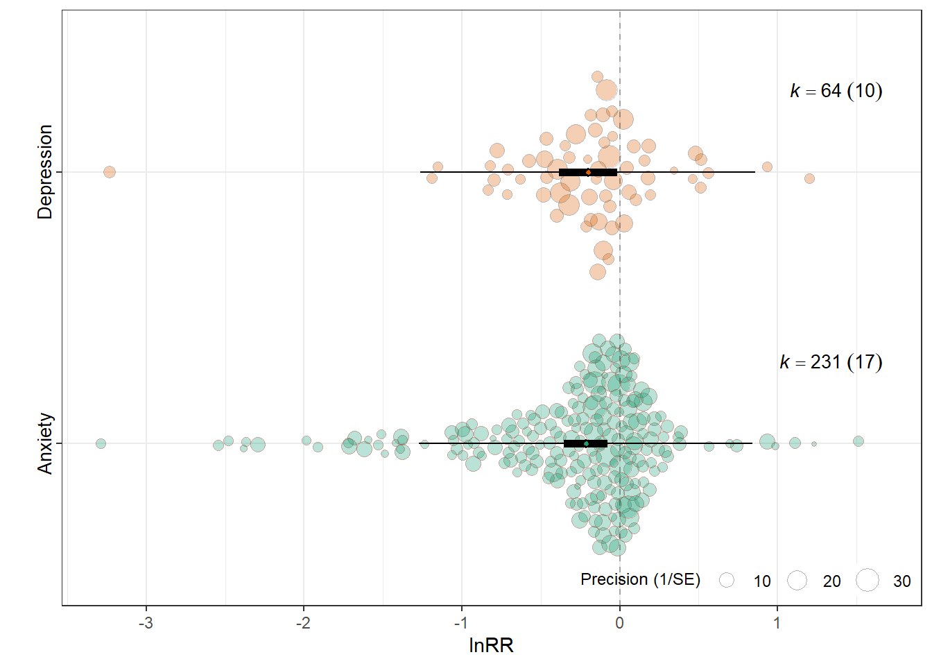
Assay type
f <- filter_low_k(db, VCV,Assay_type, min_k = 5)
db_filtered <- f$data
VCV_filtered <- f$V


mAT <- rma.mv(yi = lnRR,
                  V = VCV_filtered,
              mods = ~ Assay_type-1,
                  random = list(~1 | Study_ID,
                                ~1 | ES_ID,
                                ~1 | Strain),
                  test = "t",
                  method = "REML",
                  sparse = TRUE,
                  data = db_filtered)


assay_labels <- c(
  "Elevated Plus Maze" = "EPM",
  "Open Field Test" = "OFT",
  "Light-Dark Box" = "LDB",
  "Forced Swim Test (FST)" = "FST",
  "Tail Suspension Test (TST)" = "TST",
  "Sucrose Preference Test (SPT)" = "SPT"
)

orchard_assay <- orchard_plot(
  mAT,legend.pos = "top.left",
  mod   = "Assay_type",
  group = "Study_ID",
  xlab  = expression(lnRR),trunk.size = 0.3,
              branch.size = 2, alpha = 0.3
) +
  scale_colour_brewer(palette = "Set1") +
  scale_fill_brewer(palette = "Dark2") +
  scale_x_discrete(labels = assay_labels) +scale_y_continuous(limits = c(-4,2),breaks = seq(-4, 2, by = 1),
                                                                    minor_breaks = seq(-4, 2, by = 0.5 ))+
  labs(
    x = NULL,
    y = expression(lnRR),
    subtitle = "Behavioural assay"
  ) +
  theme(
    plot.subtitle = element_text(size = 10, face = "bold"),
    axis.title.y = element_text(face = "bold"),legend.direction = "vertical"
  )

orchard_assay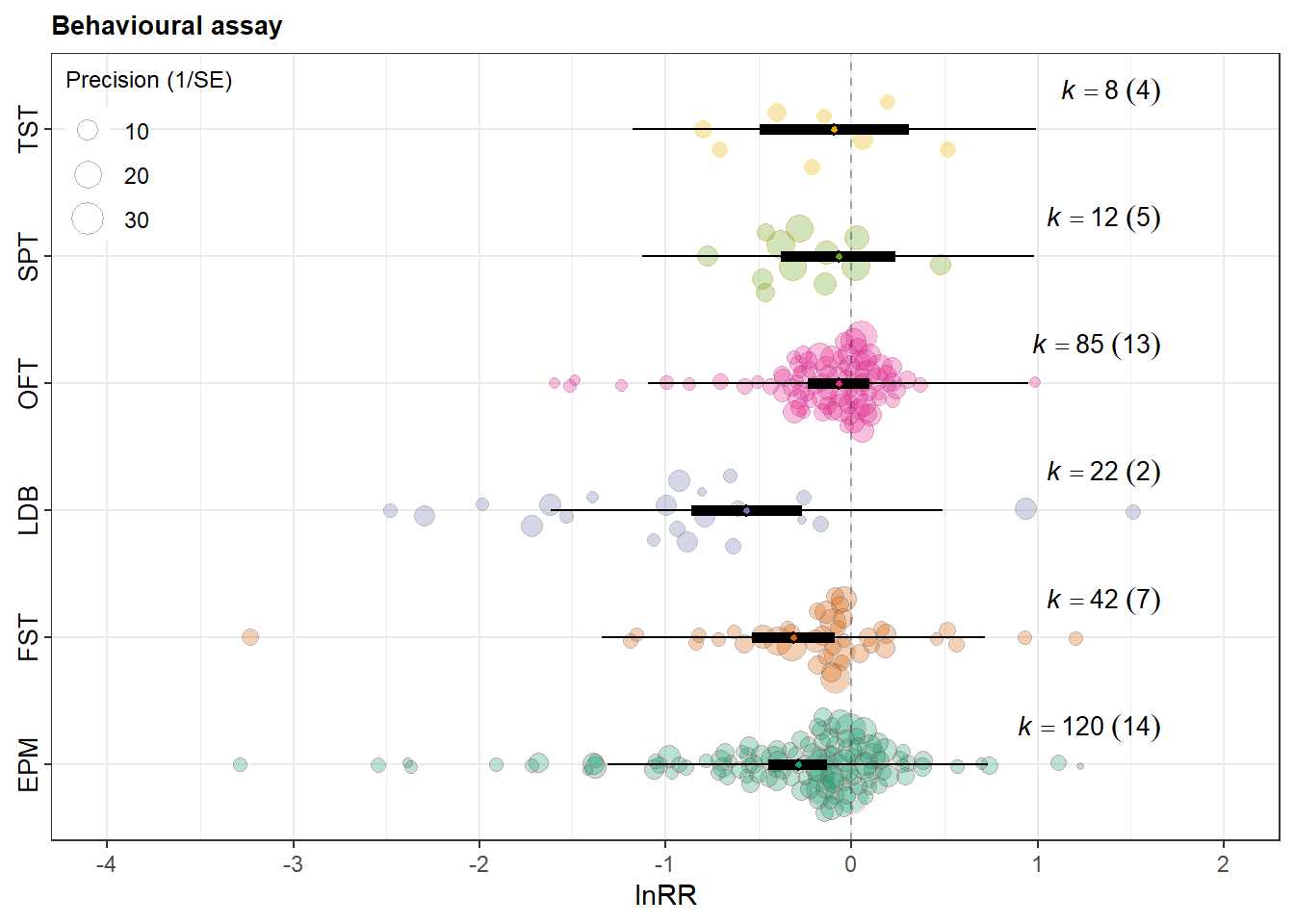
Lifestage of exposure
mLE <- rma.mv(yi = lnRR,
                  V = VCV,
              mods = ~ Lifestage_exposure-1,
                  random = list(~1 | Study_ID,
                                ~1 | ES_ID,
                                ~1 | Strain),
                  test = "t",
                  method = "REML",
                  sparse = TRUE,
                  data = db)


lifestage_labels <- c(
  "Adolescent"  = "Adol.",
  "Adult"       = "Adult",
  "Juvenile"    = "Juv.",
  "Young adult" = "Y. adult",
  "Mixed"       = "Mixed",
  "Unclear"     = "Unclear"
)


orchard_lifestage<-orchard_plot(mLE,legend.pos = "top.left",
             mod = "Lifestage_exposure",
              group = "Study_ID",
               xlab = expression(lnRR),trunk.size = 0.3,
              branch.size = 2,alpha=0.3 ,
             flip = T) +
  scale_x_discrete(labels = lifestage_labels)+
            scale_colour_brewer(palette = "Set1") +
            scale_fill_brewer(palette = "Dark2")+scale_x_discrete(labels = assay_labels) +scale_y_continuous(limits = c(-4,2),breaks = seq(-4, 2, by = 1),
                                                                    minor_breaks = seq(-4, 2, by = 0.5 ))+  theme(legend.direction = "vertical")
orchard_lifestage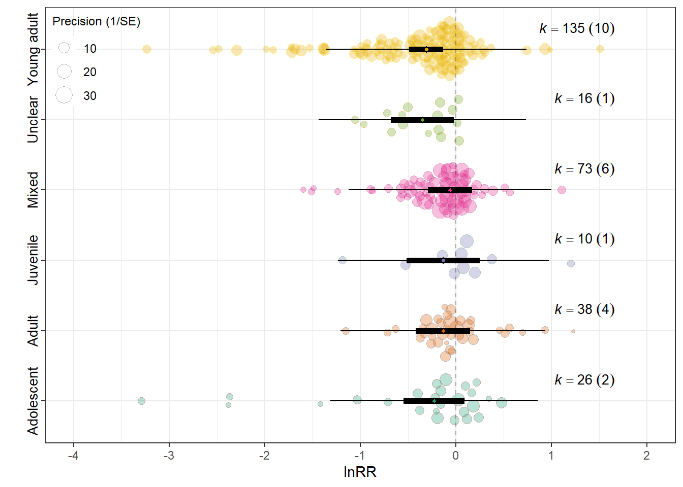
Control condition
mCC <- rma.mv(yi = lnRR,
                  V = VCV,
              mods = ~ Control_conditions,
                  random = list(~1 | Study_ID,
                                ~1 | ES_ID,
                                ~1 | Strain),
                  test = "t",
                  method = "REML",
                  sparse = TRUE,
                  data = db)


control_labels <- c(
  "ambiet sound" = "Ambient sound",
  "white noise"  = "White noise"
)
orchard_control<-orchard_plot(mCC,
             mod = "Control_conditions",legend.pos = "top.left",
              group = "Study_ID",
              xlab = expression(lnRR),trunk.size = 0.3,
              branch.size = 2,alpha=0.3) +
  scale_x_discrete(labels = control_labels) +
            scale_colour_brewer(palette = "Set1") +
            scale_fill_brewer(palette = "Dark2")+scale_x_discrete(labels = assay_labels) +scale_y_continuous(limits = c(-4,2),breaks = seq(-4, 2, by = 1),
                                                                    minor_breaks = seq(-4, 2, by = 0.5 ))+  theme(legend.direction = "vertical")
orchard_control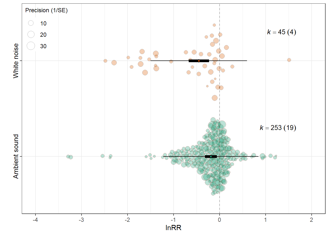
Induced behaviour
mIB <- rma.mv(yi = lnRR,
                  V = VCV,
              mods = ~ `Induced behaviour`,
                  random = list(~1 | Study_ID,
                                ~1 | ES_ID,
                                ~1 | Strain),
                  test = "t",
                  method = "REML",
                  sparse = TRUE,
                  data = db)


orchard_behaviour<-orchard_plot(mIB,
             mod = "Induced behaviour",legend.pos = "top.left",
              group = "Study_ID",
              xlab = expression(lnRR), trunk.size = 0.3,
              branch.size = 2,alpha=0.3,
              flip = T)+
            scale_colour_brewer(palette = "Set1") +
            scale_fill_brewer(palette = "Dark2")+scale_y_continuous(limits = c(-4,2),breaks = seq(-4, 2, by = 1),
                                                                    minor_breaks = seq(-4, 2, by = 0.5 ))+  theme(legend.direction = "vertical")
orchard_behaviour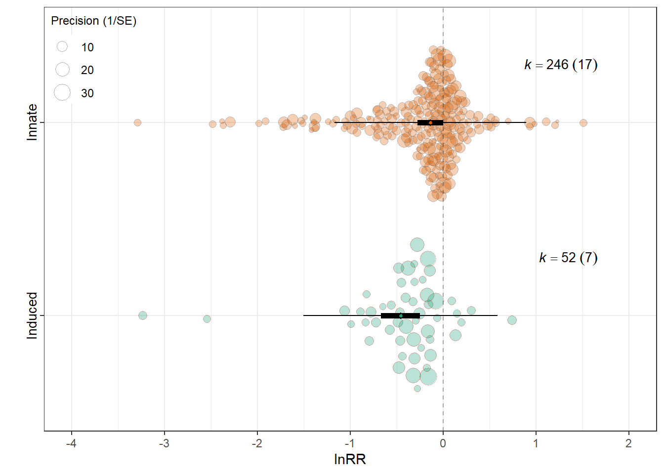
Patched figure
orchard_assay     <- orchard_assay     + labs(subtitle = "Behavioral assay")
orchard_lifestage <- orchard_lifestage + labs(subtitle = "Age at exposure")
orchard_control   <- orchard_control   + labs(subtitle = "Control condition")
orchard_behaviour <- orchard_behaviour + labs(subtitle = "Behavioral mechanism")

# 2) Hide legends on all but ONE panel (choose bottom-right here)
orchard_assay     <- orchard_assay     + theme(legend.position = "none")
orchard_lifestage <- orchard_lifestage + theme(legend.position = "none")

orchard_control   <- orchard_control   + theme(legend.position = "none")
# orchard_behaviour keeps the legend

# 3) Patch with your layout
patched_figure <- (orchard_assay + orchard_lifestage  ) /
                 (orchard_control   + orchard_behaviour) +
  plot_annotation(tag_levels = "A") &
  theme(
    plot.tag = element_text(size = 12, face = "bold"),
    plot.subtitle = element_text(size = 10, face = "bold")
  )

# 4) Enforce identical lnRR scale and a single y-axis label across ALL panels
patched_figure <- patched_figure &
  scale_y_continuous(
    limits = c(-4, 2),
    breaks = seq(-4, 2, by = 1),
    minor_breaks = seq(-4, 2, by = 0.5)
  ) &
  labs(y = expression(lnRR), x = NULL)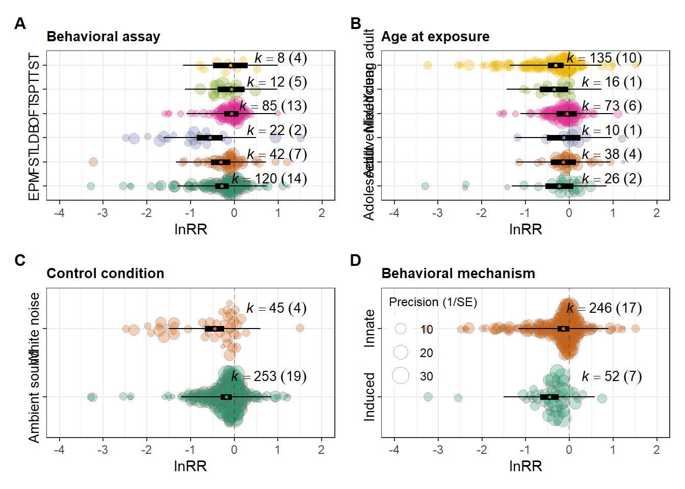
ggsave(filename = here("..","Plots", "patched_lnRR.pdf"),
       plot = patched_figure,
       dpi = 300, device = cairo_pdf,width = 10,
       height = 10)

ggsave(filename = here("..","Plots", "patched_lnRR.jpg"),
       plot = patched_figure,
       width = 10,
       height = 10,
       dpi = 300)
lnVR
db <- readr::read_csv(here("..","data","db_effect_sizes.csv")) %>%
  mutate(across(c(C_n, Ex_n, C_mean, Ex_mean, C_SE, Ex_SE, C_SD, Ex_SD, lnVR, lnVR_var), as.numeric)) %>%
  mutate(across(where(is.character), as.factor)) %>% filter(!is.na(lnVR),  !is.na(lnVR_var))


# CALCULATE VCV USING lnVR VARIANCE
VCV <- metafor::vcalc(
  vi = lnVR_var,
  cluster = Cohort_ID, # The clustering variable (Study_ID + Ex_ID)
  obs = ES_ID,         # The unique observation/effect size ID
  rho = 0.5,           # Assumed correlation between outcomes from the same cohort
  data = db
)
Overall effect
mOV <- rma.mv(yi = lnVR,
                  V = VCV,
              mods = ~ 1,
                  random = list(~1 | Study_ID,
                                ~1 | ES_ID,
                                ~1 | Strain),
                  test = "t",
                  method = "REML",
                  sparse = TRUE,
                  data = db)


orchard_overalllnVR<-orchard_plot(mOV,
               group = "Study_ID",
               xlab = "lnVR",
              flip = T,trunk.size = 0.3,
              branch.size = 2, alpha = 0.3) +
              scale_x_discrete(labels = c("Overall effect"))+
            scale_colour_brewer(palette = "Dark2") +
            scale_fill_brewer(palette = "Paired")+scale_y_continuous(limits = c(-4,11),breaks = seq(-4, 10, by = 2),
                                                                    minor_breaks = seq(-4, 11, by = 1 ))
orchard_overalllnVR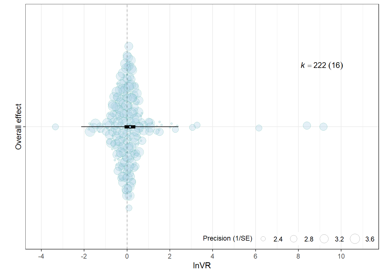
Outcome type
f <- filter_low_k(db, VCV,Outcome_type, min_k = 5)
db_filtered <- f$data
VCV_filtered <- f$V

mOT2 <- rma.mv(yi = lnVR,
                  V = VCV_filtered,
              mods = ~ Outcome_type,
                  random = list(~1 | Study_ID,
                                ~1 | ES_ID,
                                ~1 | Strain),
                  test = "t",
                  method = "REML",
                  sparse = TRUE,
                  data = db_filtered)


orchard_outcome_lnVR<-orchard_plot(mOT2,
              mod = "Outcome_type",
               group = "Study_ID",
               xlab = "lnVR",
              flip = T,trunk.size = 0.3,alpha = 0.3,
              branch.size = 2) +
            scale_colour_brewer(palette = "Dark2") +
            scale_fill_brewer(palette = "Set1")+scale_y_continuous(limits = c(-4,11),breaks = seq(-4, 10, by = 2),
                                                                    minor_breaks = seq(-4, 11, by = 1 ))
orchard_outcome_lnVR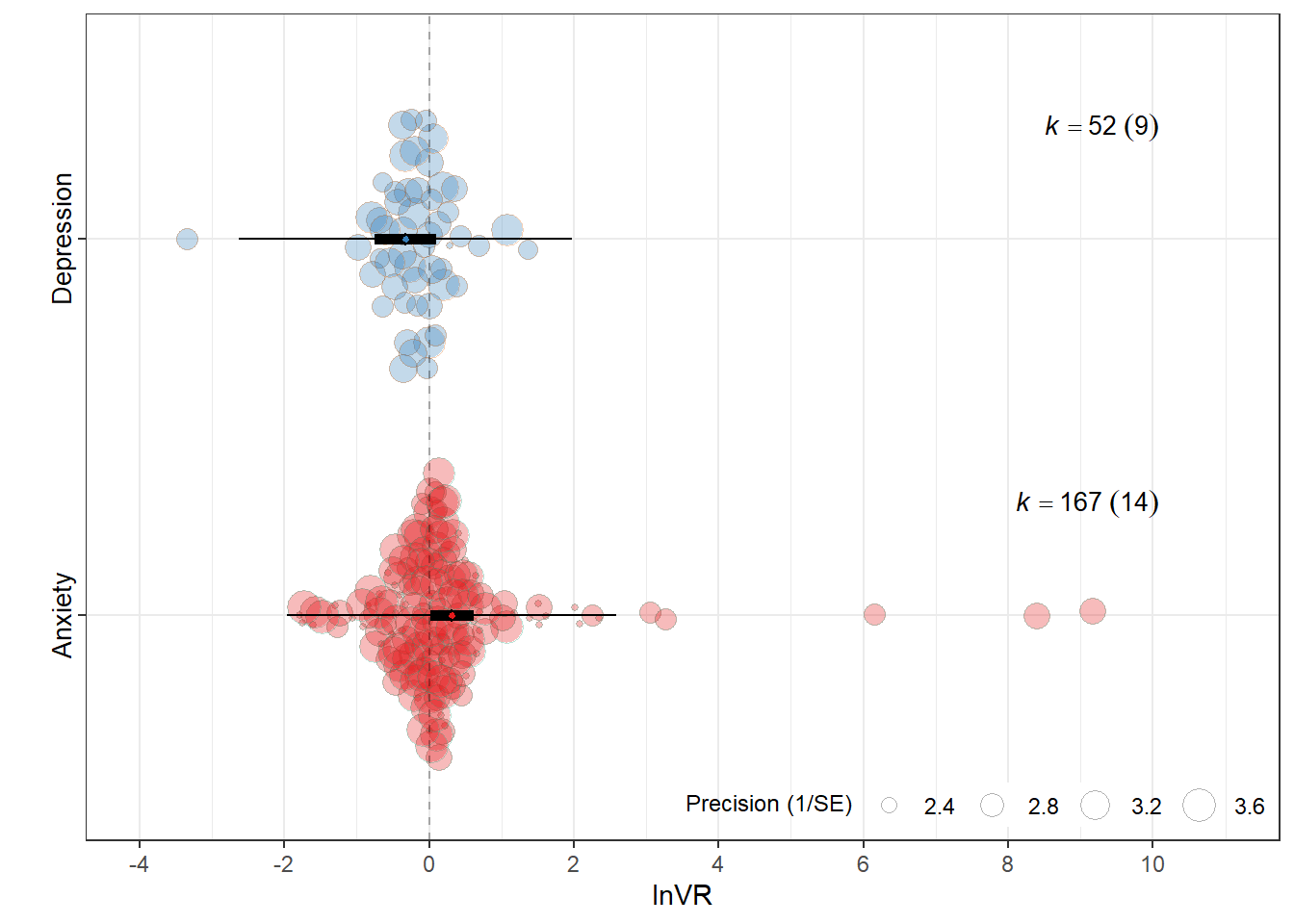
Assay type
#| label: filter_assay_type_lnVR
f <- filter_low_k(db, VCV, Assay_type, min_k = 5)
db_filtered <- f$data
VCV_filtered <- f$V


mAT <- rma.mv(yi = lnVR,
                  V = VCV_filtered,
              mods = ~ Assay_type-1,
                  random = list(~1 | Study_ID,
                                ~1 | ES_ID,
                                ~1 | Strain),
                  test = "t",
                  method = "REML",
                  sparse = TRUE,
                  data = db_filtered)


assay_labels <- c(
  "Elevated Plus Maze" = "EPM",
  "Open Field Test" = "OFT",
  "Light-Dark Box" = "LDB",
  "Forced Swim Test (FST)" = "FST",
  "Tail Suspension Test (TST)" = "TST",
  "Sucrose Preference Test (SPT)" = "SPT"
)

orchard_assay <- orchard_plot(
  mAT,legend.pos = "top.left",
  mod   = "Assay_type",
  group = "Study_ID",
  xlab  = expression(lnVR) ,trunk.size = 0.3,
              branch.size = 2,alpha = 0.3
) +
  scale_colour_brewer(palette = "Set1") +
  scale_fill_brewer(palette = "Dark2") +
  scale_x_discrete(labels = assay_labels)+
  scale_y_continuous(limits = c(-4,11),breaks = seq(-4, 11, by = 2),
                     minor_breaks = seq(-4, 11, by = 1 ))+
  labs(
    x = NULL,
    y = expression(lnVR),
    subtitle = "Behavioural assay"
  ) +
  theme(
    plot.subtitle = element_text(size = 10, face = "bold"),
    axis.title.y = element_text(face = "bold"),legend.direction = "vertical")


orchard_assay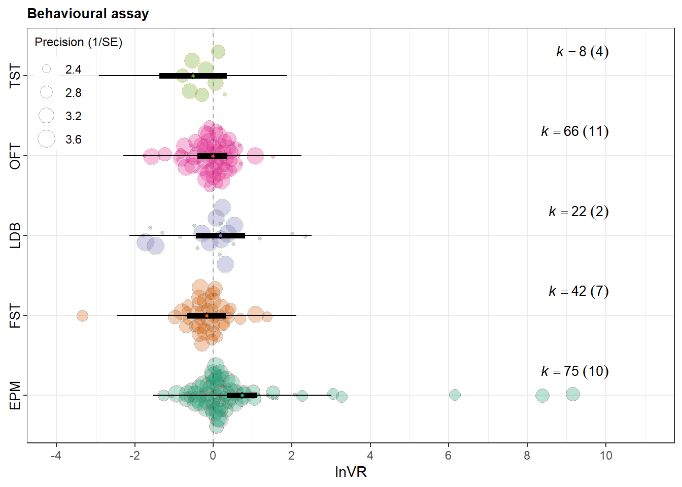
Lifestage of exposure
mLE <- rma.mv(yi = lnVR,
                  V = VCV,
              mods = ~ Lifestage_exposure-1,
                  random = list(~1 | Study_ID,
                                ~1 | ES_ID,
                                ~1 | Strain),
                  test = "t",
                  method = "REML",
                  sparse = TRUE,
                  data = db)


lifestage_labels <- c(
  "Adolescent"  = "Adol.",
  "Adult"       = "Adult",
  "Juvenile"    = "Juv.",
  "Young adult" = "Y. adult",
  "Mixed"       = "Mixed",
  "Unclear"     = "Unclear"
)


orchard_lifestage<-orchard_plot(mLE,legend.pos = "top.left",
              mod = "Lifestage_exposure",
               group = "Study_ID",
                xlab = expression(lnVR), trunk.size = 0.3,
              branch.size = 2 ,alpha = 0.3
              ) + scale_x_discrete(labels = lifestage_labels)+
            scale_colour_brewer(palette = "Set1") +
            scale_fill_brewer(palette = "Dark2")+scale_y_continuous(limits=c(-4,11),breaks = seq(-4, 11, by = 2),
                                                                    minor_breaks = seq(-4, 11, by = 1 ))+
  theme(legend.direction = "vertical")
orchard_lifestage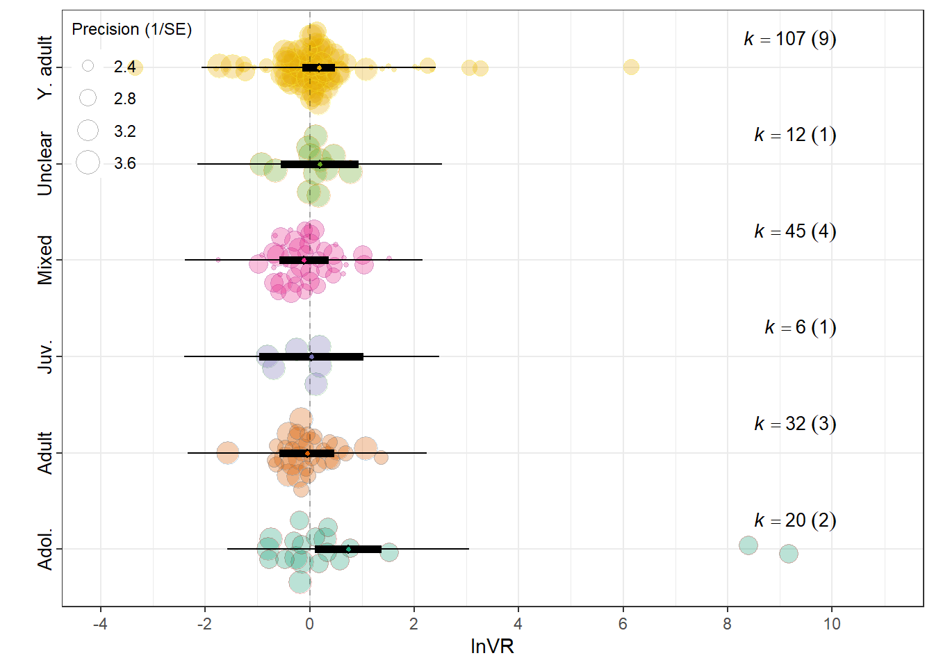
Music genre
Meta_genre
mMG <- rma.mv(yi = lnVR,
                  V = VCV,
              mods = ~ Meta_genre-1 ,
                  random = list(~1 | Study_ID,
                                ~1 | ES_ID,
                                ~1 | Strain),
                  test = "t",
                  method = "REML",
                  sparse = TRUE,
                  data = db)


genre_labels <- c(
  "Mixed"  = "Mixed",
  "Popular Contemporary Music"       = "Contemporary",
  "Traditional Music / Folk / World"    = "World",
  "Western Art Music / Orchestral" = "Orchestral"
)


orchard_genre<-orchard_plot(mMG,legend.pos = "top.left",
             mod = "Meta_genre",
              group = "Study_ID",
             xlab = "lnVR",
             flip = T,trunk.size = 0.3,
              branch.size = 2,alpha = 0.3) +
  scale_x_discrete(labels = genre_labels)+
            scale_colour_brewer(palette = "Set1") +
            scale_fill_brewer(palette = "Dark2")+scale_y_continuous(limits=c(-4,11),breaks = seq(-4, 11, by = 2),
                                                                    minor_breaks = seq(-4, 11, by = 1 ))+
  theme(legend.direction = "vertical")
orchard_genre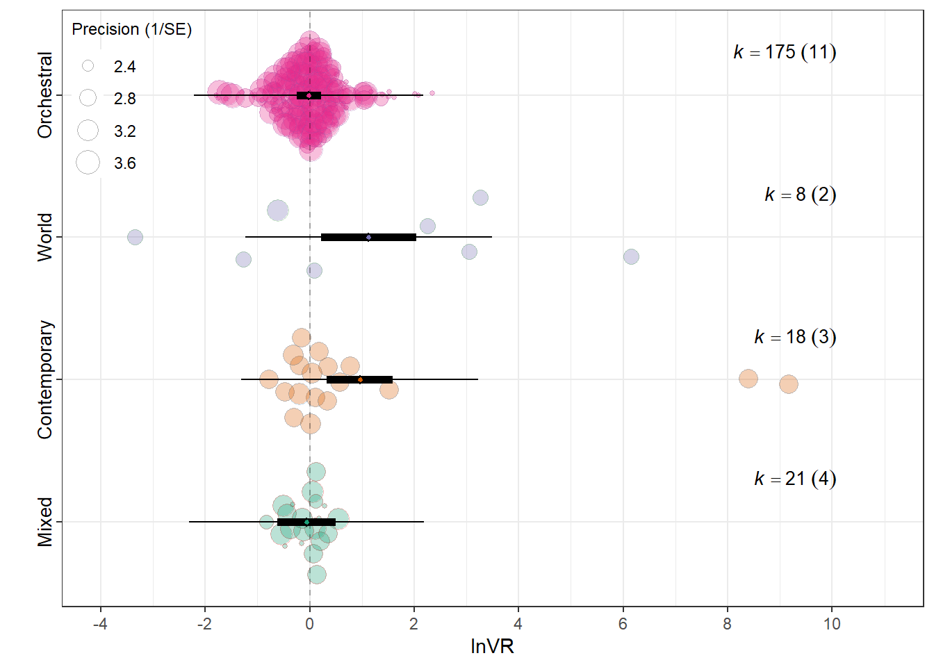
Experimental design
mEXD <- rma.mv(yi = lnVR,
                  V = VCV,
              mods = ~ Experimental_design-1,
                  random = list(~1 | Study_ID,
                                ~1 | ES_ID,
                                ~1 | Strain),
                  test = "t",
                  method = "REML",
                  sparse = TRUE,
                  data = db)


design_labels<-c(
  "Factorial"="Factorial",
  "Posttest-Only Control Group"="Posttest",
  "Repeated Measures"="Repeated"

)


orchard_design<-orchard_plot(mEXD,legend.pos = "top.left",
             mod = "Experimental_design",
              group = "Study_ID",
              xlab = expression(lnVR),
              flip=T,
             trunk.size = 0.3,
              branch.size = 2,alpha = 0.3 ) +
  scale_x_discrete(labels = design_labels) +
            scale_colour_brewer(palette = "Set1") +
            scale_fill_brewer(palette = "Dark2")+scale_y_continuous(limits = c(-4,11),breaks = seq(-4, 11, by = 2),
                                                                    minor_breaks = seq(-4, 11, by = 1 ))+
  theme(legend.direction = "vertical")
orchard_design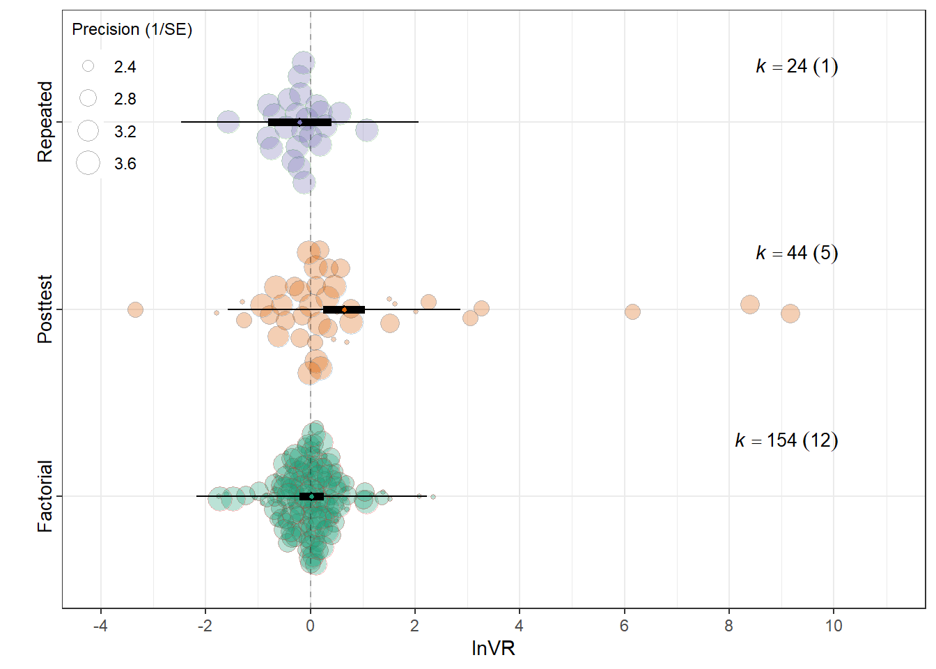
orchard_assay     <- orchard_assay     + labs(subtitle = "Behavioral assay")
orchard_lifestage <- orchard_lifestage + labs(subtitle = "Age at exposure")

orchard_genre   <- orchard_genre  + labs(subtitle = "Music meta-genre")
orchard_design <-orchard_design + labs(subtitle = "Experimental design")


# 2) Hide legends on all but ONE panel
orchard_assay    <- orchard_assay    + theme(legend.position = "none")
orchard_lifestage <- orchard_lifestage + theme(legend.position = "none")
orchard_genre   <- orchard_genre+ theme(legend.position = "none")

# orchard_behaviour keeps the legend

# 3) Patch with your layout
patched_figure <- ( orchard_assay+orchard_lifestage) /
                 (orchard_genre + orchard_design) +
  plot_annotation(tag_levels = "A") &
  theme(
    plot.tag = element_text(size = 12, face = "bold"),
    plot.subtitle = element_text(size = 10, face = "bold")
   )


# 4) Enforce identical lnRR scale and a single y-axis label across ALL panels
patched_figure <- patched_figure &
  scale_y_continuous(
    limits = c(-4, 11),
    breaks = seq(-4, 11, by = 2),
    minor_breaks = seq(-4, 11, by = 1)
  ) &
  labs(y = expression(lnVR), x = NULL)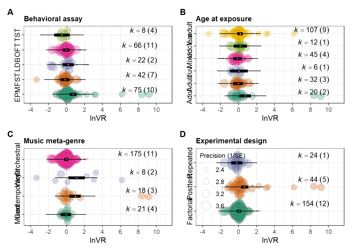
ggsave(filename = here("..","Plots", "patched_lnVR.pdf"),
       plot = patched_figure,
       dpi = 300, device = cairo_pdf,width = 10,
       height = 10)

ggsave(filename = here("..","Plots", "patched_lnVR.jpg"),
       plot = patched_figure,
       width = 10,
       height = 10,
       dpi = 300)
Overall effects figure
fig2<-(overall_lnRR/orchard_overalllnVR)

fig2<-fig2+
  plot_annotation(
    title = '',
    tag_levels = 'A'
  )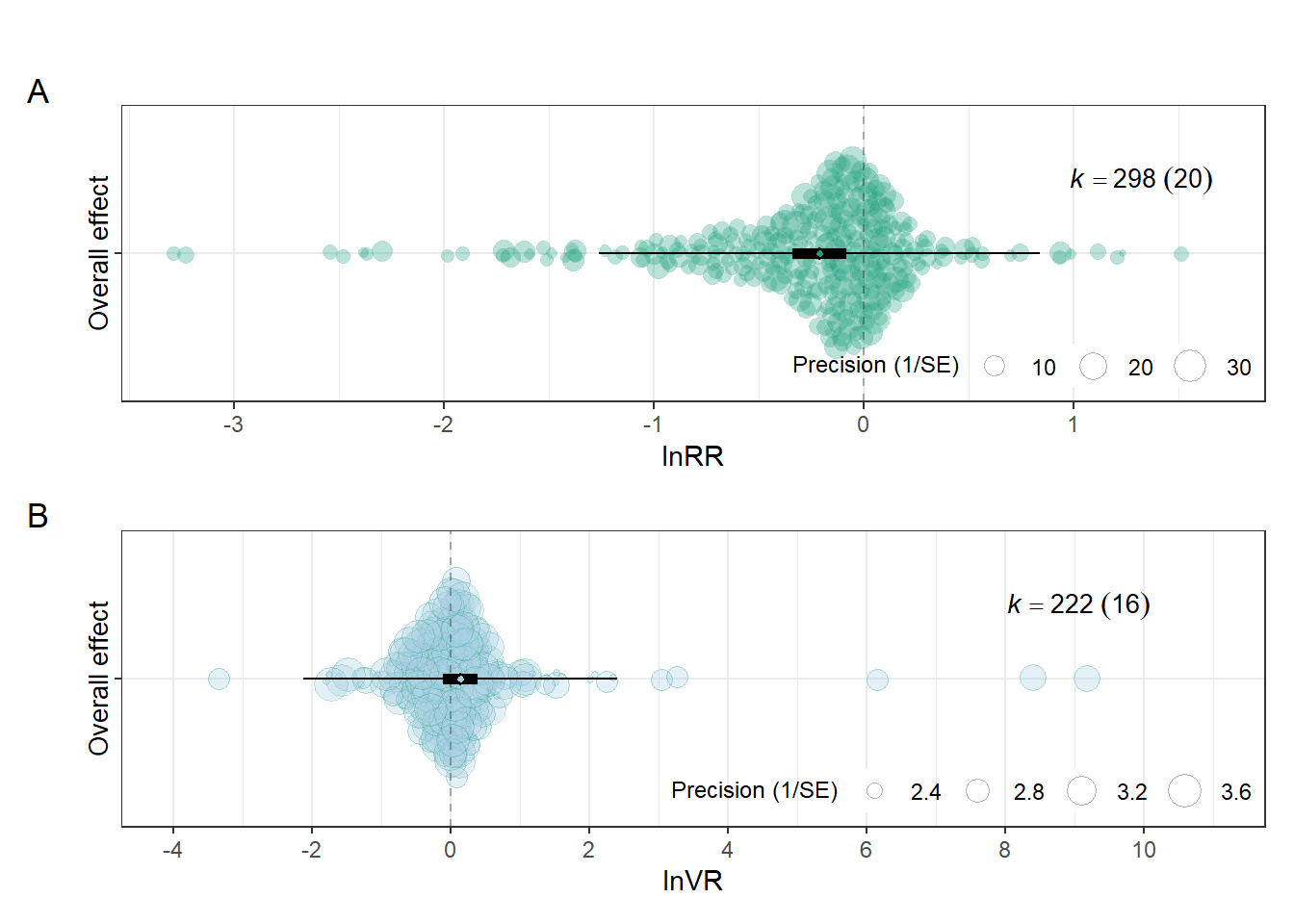
ggsave(filename = here("..","Plots", "overall_effects.pdf"),
       plot = fig2,
       dpi = 300, device = cairo_pdf)

ggsave(filename = here("..","Plots", "overall_effects.jpg"),
       plot = fig2,
       width = 7,
       height = 9,
       dpi = 300)
Outcome type figure
fig3<-(orchard_outcomelnRR/orchard_outcome_lnVR)

fig3<-fig3+
  plot_annotation(
    title = '',
    tag_levels = 'A'
  )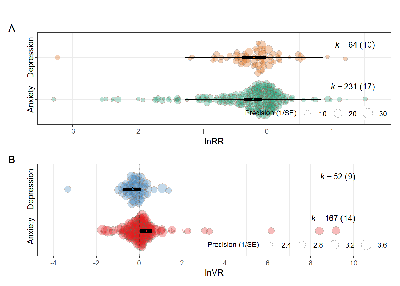
ggsave(filename = here("..","Plots", "outcome_effects.pdf"),
       plot = fig3,
       dpi = 300, device = cairo_pdf)

ggsave(filename = here("..","Plots", "outcome_effects.jpg"),
       plot = fig3,
       width = 7,
       height = 9,
       dpi = 300)