---
title: "Descriptive summaries"
---
::: {.workflow}
::: {}
**Input**
Saved SAFE lnM dataset.
:::
::: {}
**Action**
Count the 7,186 analysed (m00) contrasts and draw data-distribution plots.
:::
::: {}
**Output**
Descriptive tables, plots, and CSV files.
:::
::: {}
**Next**
Check associations among moderators.
:::
:::
```{r setup}
source(here::here("Scripts", "00_packages.R"))
source(here::here("Scripts", "01_paths.R"))

theme_descriptive <- function() {
  ggplot2::theme_classic(base_size = 12) +
    ggplot2::theme(
      plot.title = ggplot2::element_text(face = "bold", hjust = 0.5),
      axis.line = ggplot2::element_blank(),
      axis.ticks = ggplot2::element_blank(),
      axis.text = ggplot2::element_blank(),
      axis.title = ggplot2::element_blank(),
      legend.title = ggplot2::element_blank()
    )
}

plot_count_donut <- function(dat, var, title, palette = NULL) {
  count_dat <- dat |>
    dplyr::filter(!is.na(.data[[var]])) |>
    dplyr::count(.data[[var]], name = "n", sort = TRUE) |>
    dplyr::mutate(
      prop = n / sum(n),
      label = stringr::str_wrap(paste0(.data[[var]], " (", n, ")"), width = 24),
      ypos = cumsum(prop) - 0.5 * prop
    )

  if (is.null(palette)) {
    palette <- scales::hue_pal(l = 58, c = 70)(nrow(count_dat))
  }

  ggplot2::ggplot(count_dat, ggplot2::aes(x = 2, y = prop, fill = label)) +
    ggplot2::geom_col(width = 1, colour = "white", linewidth = 0.5) +
    ggplot2::coord_polar(theta = "y") +
    ggplot2::xlim(0.5, 2.5) +
    ggplot2::scale_fill_manual(values = palette) +
    ggplot2::labs(title = title, fill = NULL) +
    ggplot2::annotate(
      "text",
      x = 0.5,
      y = 0,
      label = paste0("k = ", sum(count_dat$n)),
      fontface = "bold",
      size = 4
    ) +
    ggplot2::guides(fill = ggplot2::guide_legend(ncol = 2, byrow = TRUE)) +
    theme_descriptive()
}
```
## Input: load effect-size dataset
```{r load}
dat_es <- readRDS(here::here("Rdata", "effect_sizes", "proceed_lnm_safe.rds"))
m00_fit <- readRDS(
  here::here("Rdata", "models", "m00_ls_intercept_only.rds")
)
name_map <- readRDS(
  here::here("Rdata", "phylogeny", "proceed_name_map.rds")
)
canonical_lookup <- stats::setNames(
  as.character(name_map$sp_ncbi_canonical),
  as.character(name_map$sp_ncbi_original)
)

# The model data renumber es_id_model 1..k after rows without a canonical
# species name are dropped (Scripts/05_phylogeny.R), so the IDs cannot be
# matched back to dat_es directly. Rebuild the same filter, keeping row order,
# and verify it row by row against the data stored in the m00 fit.
dat_es_canonical <- unname(canonical_lookup[as.character(dat_es$sp_ncbi)])
m00_dat <- dat_es[
  !is.na(dat_es_canonical) & nzchar(dat_es_canonical), , drop = FALSE
]
m00_check <- nrow(m00_dat) == nrow(m00_fit$data) &&
  isTRUE(all.equal(m00_dat$yi_lnM_safe, m00_fit$data$yi_lnM_safe)) &&
  identical(as.character(m00_dat$ref_id), as.character(m00_fit$data$ref_id)) &&
  identical(
    unname(canonical_lookup[as.character(m00_dat$sp_ncbi)]),
    as.character(m00_fit$data$sp_ncbi)
  )

if (!m00_check) {
  stop("The descriptive dataset does not reproduce the rows retained by m00.")
}

cat("SAFE contrasts:", nrow(dat_es), "\n")
cat("m00 contrasts:", nrow(m00_dat), "\n")
cat("Excluded before modelling:", nrow(dat_es) - nrow(m00_dat), "\n")
```
All counts, tables, donut plots, and distributions in this chapter describe
the analysed dataset: the `r scales::comma(nrow(m00_dat))` contrasts retained
by the baseline model `m00`. The saved SAFE dataset contains
`r scales::comma(nrow(dat_es))` contrasts; the
`r nrow(dat_es) - nrow(m00_dat)` contrasts whose species names could not be
resolved were excluded before modelling and are not counted here.
## Check: overview counts
```{r overview}
m00_dat |>
  dplyr::summarise(
    k_contrasts  = dplyr::n(),
    n_studies    = dplyr::n_distinct(ref_id),
    n_systems    = dplyr::n_distinct(sys_id),
    n_species    = dplyr::n_distinct(canonical_lookup[as.character(sp_ncbi)]),
    n_allochronic = sum(design == "Allochronic", na.rm = TRUE),
    n_synchronic  = sum(design == "Synchronic",  na.rm = TRUE)
  )
```
## Counts by moderator
The tables report the exact counts among the `r scales::comma(nrow(m00_dat))`
analysed contrasts. The plots display the same category totals.
```{r by-disturbance}
m00_dat |> dplyr::count(disturbance, sort = TRUE)
```
## Analytical coverage and evidence pathways
The baseline analysis retained `r scales::comma(nrow(m00_dat))` contrasts from
`r dplyr::n_distinct(m00_dat$ref_id)` references and
`r scales::comma(dplyr::n_distinct(m00_dat$sys_id))` study systems. After
taxonomic reconciliation, these contrasts represented
`r dplyr::n_distinct(m00_fit$data$sp_ncbi)` species. The table and figure below
use only these model-retained contrasts; their denominator therefore agrees
with the sample size reported for `m00`.
```{r}
#| label: tbl-m00-coverage
#| tbl-cap: "Coverage of the baseline analytical sample. Percentages are the share of all 7,186 contrasts retained by m00."
coverage_variables <- c(
  disturbance = "Disturbance context",
  design = "Comparison design",
  trait_type = "Trait type",
  genphen = "Evidence type",
  taxa = "Taxonomic group"
)

m00_coverage <- purrr::imap_dfr(coverage_variables, function(dimension, variable) {
  m00_dat |>
    dplyr::transmute(category = as.character(.data[[variable]])) |>
    dplyr::mutate(category = dplyr::coalesce(category, "Not reported")) |>
    dplyr::count(category, name = "Contrasts", sort = TRUE) |>
    dplyr::mutate(
      Dimension = dimension,
      `Coverage (%)` = 100 * Contrasts / nrow(m00_dat)
    ) |>
    dplyr::select(Dimension, Category = category, Contrasts, `Coverage (%)`)
})

m00_coverage |>
  dplyr::mutate(
    Contrasts = scales::comma(Contrasts),
    `Coverage (%)` = sprintf("%.1f", `Coverage (%)`)
  ) |>
  knitr::kable(
    align = c("l", "l", "r", "r"),
    col.names = c("Dimension", "Category", "Contrasts", "Coverage (%)")
  ) |>
  kableExtra::kable_styling(
    bootstrap_options = c("striped", "hover", "condensed", "responsive"),
    full_width = TRUE
  ) |>
  kableExtra::collapse_rows(columns = 1, valign = "top")
```
```{r by-design}
m00_dat |> dplyr::count(design, sort = TRUE)
```
```{r by-trait-type}
m00_dat |> dplyr::count(trait_type, sort = TRUE)
```
```{r by-taxa}
m00_dat |> dplyr::count(taxa, sort = TRUE)
```
## Taxonomic representation
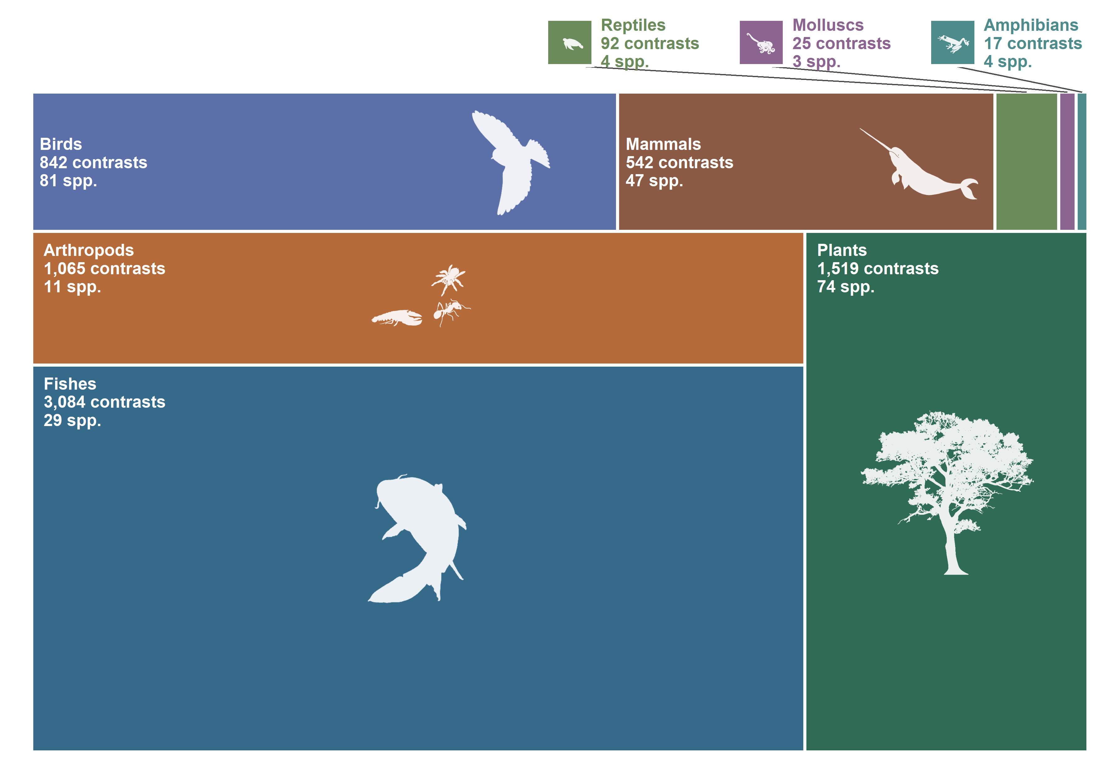
This figure counts the unique species and contrasts used by the baseline model (`m00`). Tile area is proportional to the number of contrasts in each taxonomic group. Each label gives the contrast count and species count. Groups whose tiles are too small to hold a label (reptiles, molluscs and amphibians) are labelled above the chart and joined to their tiles by leader lines. Records from the complete PROCEED database that were not included in the model are not counted.
```{r}
#| label: fig-taxonomic-representation
#| fig-cap: "Taxonomic representation in model m00. Tile area is proportional to the number of contrasts in each taxonomic group. Labels give the number of contrasts and species in each group; the three smallest groups are labelled above the chart."
#| fig-alt: "A proportional tile chart of the 7,186 m00 contrasts: fishes 3,084 contrasts (29 species), plants 1,519 (74), arthropods 1,065 (11), birds 842 (81), mammals 542 (47), reptiles 92 (4), molluscs 25 (3), and amphibians 17 (4). Each tile includes a white taxon silhouette; the three smallest groups are labelled above the chart with leader lines."
#| fig-width: 12
#| fig-height: 8.2
# Read the exact species names used by the baseline model.
m00_species <- unique(as.character(m00_fit$data$sp_ncbi))

# canonical_lookup (built in the load chunk) connects the original species
# names to the canonical names used by m00.

# Keep the exact contrasts used by m00 and count species and contrasts.
taxon_counts <- m00_dat |>
  dplyr::mutate(
    sp_ncbi_canonical = unname(canonical_lookup[as.character(sp_ncbi)])
  ) |>
  dplyr::filter(
    !is.na(taxa)
  ) |>
  dplyr::group_by(taxa) |>
  dplyr::summarise(
    species = dplyr::n_distinct(sp_ncbi_canonical, na.rm = TRUE),
    contrasts = dplyr::n(),
    .groups = "drop"
  ) |>
  dplyr::filter(species > 0) |>
  dplyr::mutate(
    taxa = as.character(taxa),
    # Tile area is proportional to the number of contrasts in each group.
    weight = contrasts
  )

# Use a wide layout. Smaller groups share a full-width strip at the top; the
# smallest groups sit at its right-hand end and are labelled outside the chart.
make_taxon_layout <- function(dat, total_width = 1.6) {
  small_order <- c("Bird", "Mammal", "Reptile", "Mollusc", "Amphibian")
  left_order <- c("Fish", "Arthropod")
  right_order <- c("Plant")
  total_weight <- sum(dat$weight)

  small <- dat[match(small_order, dat$taxa), , drop = FALSE]
  small_height <- sum(small$weight) / total_weight
  small_widths <- total_width * small$weight / sum(small$weight)
  small$xmin <- c(0, head(cumsum(small_widths), -1))
  small$xmax <- cumsum(small_widths)
  small$ymin <- 1 - small_height
  small$ymax <- 1

  large_height <- 1 - small_height
  large <- dat[dat$taxa %in% c(left_order, right_order), , drop = FALSE]
  left <- large[match(left_order, large$taxa), , drop = FALSE]
  right <- large[match(right_order, large$taxa), , drop = FALSE]
  left_width <- total_width * sum(left$weight) / sum(large$weight)

  stack_column <- function(x, xmin, xmax) {
    heights <- large_height * x$weight / sum(x$weight)
    x$xmin <- xmin
    x$xmax <- xmax
    x$ymin <- c(0, head(cumsum(heights), -1))
    x$ymax <- cumsum(heights)
    x
  }

  dplyr::bind_rows(
    stack_column(left, 0, left_width),
    stack_column(right, left_width, total_width),
    small
  )
}

taxon_tiles <- make_taxon_layout(taxon_counts) |>
  dplyr::mutate(
    area = (xmax - xmin) * (ymax - ymin),
    taxa_plural = dplyr::recode(
      taxa,
      Bird = "Birds", Plant = "Plants", Mammal = "Mammals", Fish = "Fishes",
      Arthropod = "Arthropods", Amphibian = "Amphibians",
      Reptile = "Reptiles", Mollusc = "Molluscs"
    ),
    label = paste0(
      taxa_plural, "\n",
      scales::comma(contrasts), " contrasts\n",
      species, " spp."
    ),
    is_small = taxa %in% c("Bird", "Mammal"),
    # Tiles too small to hold a label are keyed above the chart instead.
    is_external = taxa %in% c("Reptile", "Mollusc", "Amphibian"),
    label_size = 13 / ggplot2::.pt,
    label_x = xmin + ifelse(is_small, 0.012, 0.018),
    label_y = ifelse(is_small, (ymin + ymax) / 2, ymax - 0.018),
    label_vjust = ifelse(is_small, 0.5, 1)
  )

# Keys for the smallest groups: a coloured square carrying the silhouette, a
# label to its right, and a leader line from the tile's top edge to the key.
key_side <- 0.07
key_ymin <- 1.04
external_keys <- taxon_tiles |>
  dplyr::filter(is_external) |>
  dplyr::mutate(
    key_xmin = c(Reptile = 0.78, Mollusc = 1.07, Amphibian = 1.36)[taxa],
    key_xmax = key_xmin + key_side,
    key_ymin = key_ymin,
    key_ymax = key_ymin + key_side,
    leader_x = (xmin + xmax) / 2,
    leader_y = ymax,
    leader_xend = key_xmin + key_side / 2,
    leader_yend = key_ymin,
    key_label_x = key_xmax + 0.012,
    key_label_y = key_ymin + key_side / 2
  )

# Read the supplied silhouettes from Rdata/figures/Animals.
animal_dir <- here::here("Rdata", "figures", "Animals")
icon_paths <- c(
  Bird = file.path(animal_dir, "Bird.png"),
  Plant = file.path(animal_dir, "Tree.png"),
  Mammal = file.path(animal_dir, "Mammals.png"),
  Fish = file.path(animal_dir, "Fish.png"),
  Arthropod = file.path(animal_dir, "Arthropods.png"),
  Amphibian = file.path(animal_dir, "Frog.png"),
  Reptile = file.path(animal_dir, "Turtle2.png"),
  Mollusc = file.path(animal_dir, "Mollusca.png")
)

read_white_silhouette <- function(path) {
  image <- png::readPNG(path)
  if (dim(image)[3] == 4) {
    alpha <- image[, , 4]
  } else {
    brightness <- apply(image[, , 1:3, drop = FALSE], c(1, 2), mean)
    alpha <- pmin(1, pmax(0, (1 - brightness) * 8))
  }
  white <- array(1, dim = c(dim(image)[1], dim(image)[2], 4))
  white[, , 4] <- alpha * 0.90
  white
}

internal_tiles <- dplyr::filter(taxon_tiles, !is_external)

icon_layers <- lapply(seq_len(nrow(internal_tiles)), function(i) {
  tile <- internal_tiles[i, ]
  image <- read_white_silhouette(icon_paths[[tile$taxa]])
  tile_width <- tile$xmax - tile$xmin
  tile_height <- tile$ymax - tile$ymin
  image_ratio <- dim(image)[2] / dim(image)[1]
  keep_size <- tile$taxa %in% c("Fish", "Arthropod")
  max_width <- tile_width * ifelse(
    keep_size, 0.48,
    ifelse(tile$is_small, 0.34, 0.62)
  )
  max_height <- tile_height * ifelse(
    keep_size, 0.55,
    ifelse(tile$is_small, 0.84, 0.68)
  )
  icon_width <- min(max_width, max_height * image_ratio)
  icon_height <- icon_width / image_ratio
  centre_x <- ifelse(
    tile$is_small,
    tile$xmax - tile_width * 0.20,
    (tile$xmin + tile$xmax) / 2
  )
  centre_y <- (tile$ymin + tile$ymax) / 2

  ggplot2::annotation_custom(
    grid::rasterGrob(image, interpolate = TRUE),
    xmin = centre_x - icon_width / 2,
    xmax = centre_x + icon_width / 2,
    ymin = centre_y - icon_height / 2,
    ymax = centre_y + icon_height / 2
  )
})

key_icon_layers <- lapply(seq_len(nrow(external_keys)), function(i) {
  key <- external_keys[i, ]
  image <- read_white_silhouette(icon_paths[[key$taxa]])
  image_ratio <- dim(image)[2] / dim(image)[1]
  icon_width <- min(key_side * 0.80, key_side * 0.80 * image_ratio)
  icon_height <- icon_width / image_ratio
  centre_x <- (key$key_xmin + key$key_xmax) / 2
  centre_y <- (key$key_ymin + key$key_ymax) / 2

  ggplot2::annotation_custom(
    grid::rasterGrob(image, interpolate = TRUE),
    xmin = centre_x - icon_width / 2,
    xmax = centre_x + icon_width / 2,
    ymin = centre_y - icon_height / 2,
    ymax = centre_y + icon_height / 2
  )
})

taxon_colours <- c(
  Bird = "#5B6FA8", Plant = "#2F6B55", Mammal = "#8A5A44",
  Fish = "#356A8A", Arthropod = "#B56A3A", Amphibian = "#4E8C8C",
  Reptile = "#6C8B5A", Mollusc = "#8B648F"
)

p_taxa <- ggplot2::ggplot(taxon_tiles) +
  ggplot2::geom_rect(
    ggplot2::aes(xmin = xmin, xmax = xmax, ymin = ymin, ymax = ymax, fill = taxa),
    colour = "white", linewidth = 1.2
  )

p_taxa <- p_taxa +
  ggplot2::geom_segment(
    data = external_keys,
    ggplot2::aes(x = leader_x, y = leader_y,
                 xend = leader_xend, yend = leader_yend),
    colour = "#4A4A4A", linewidth = 0.45
  ) +
  ggplot2::geom_rect(
    data = external_keys,
    ggplot2::aes(xmin = key_xmin, xmax = key_xmax,
                 ymin = key_ymin, ymax = key_ymax, fill = taxa),
    colour = "white", linewidth = 1.2
  )

for (icon_layer in c(icon_layers, key_icon_layers)) {
  p_taxa <- p_taxa + icon_layer
}

p_taxa <- p_taxa +
  ggplot2::geom_text(
    data = internal_tiles,
    ggplot2::aes(x = label_x, y = label_y, label = label,
                 size = label_size, vjust = label_vjust),
    colour = "white", fontface = "bold", hjust = 0,
    lineheight = 0.9
  ) +
  ggplot2::geom_text(
    data = external_keys,
    ggplot2::aes(x = key_label_x, y = key_label_y, label = label,
                 size = label_size, colour = taxa),
    fontface = "bold", hjust = 0, vjust = 0.5, lineheight = 0.9
  ) +
  ggplot2::scale_fill_manual(values = taxon_colours) +
  ggplot2::scale_colour_manual(values = taxon_colours) +
  ggplot2::scale_size_identity() +
  ggplot2::coord_fixed(
    ratio = 1, xlim = c(0, 1.6), ylim = c(0, key_ymin + key_side + 0.01),
    expand = FALSE, clip = "off"
  ) +
  ggplot2::theme_void(base_size = 13) +
  ggplot2::theme(
    legend.position = "none",
    plot.margin = ggplot2::margin(10, 10, 10, 10)
  )

# Save the same figure displayed below.
ggplot2::ggsave(
  here::here("Rdata", "figures", "taxonomic_representation.png"),
  p_taxa, width = 12, height = 8.2, dpi = 320, bg = "white"
)
ggplot2::ggsave(
  here::here("Figures", "taxonomic_representation.pdf"),
  p_taxa, width = 12, height = 8.2, device = grDevices::cairo_pdf,
  bg = "white"
)

p_taxa
```
### Evidence pathways
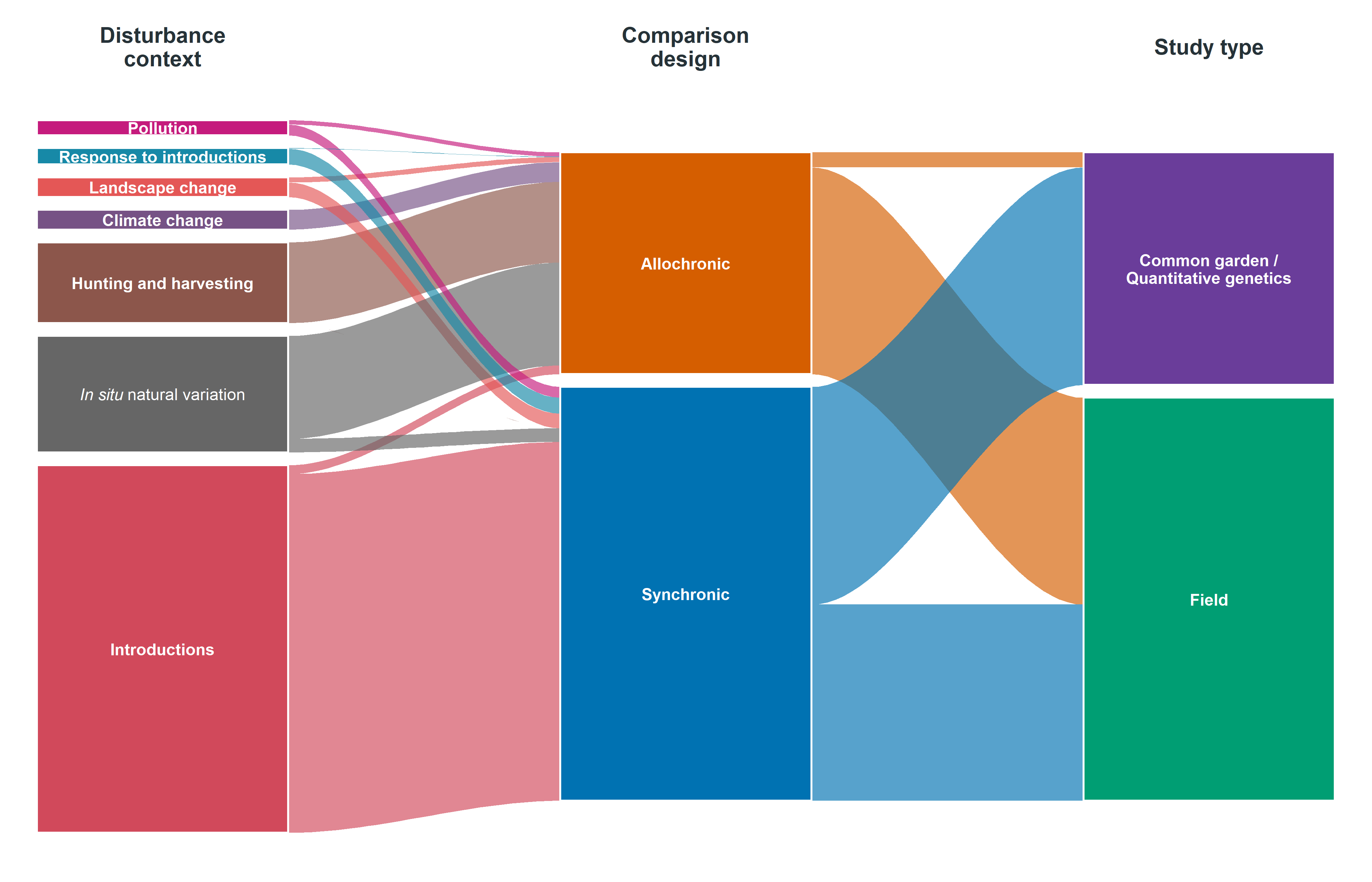
Flow width is proportional to the number of `m00` contrasts following each
path. Colour identifies disturbance context at the first axis and is carried
through the remaining axes. Counts and percentages are reported in
@tbl-m00-coverage rather than repeated inside the figure.
```{r}
#| label: fig-m00-alluvial-coverage
#| fig-cap: "Evidence pathways among the 7,186 contrasts retained by model m00, from disturbance context through comparison design to study type. Flow width is proportional to the number of contrasts."
#| fig-alt: "An alluvial plot beginning with disturbance contexts, passing through synchronic and allochronic comparison designs, and ending with field or common-garden and quantitative-genetic study types."
#| fig-width: 14
#| fig-height: 9
make_alluvial <- function(dat, axes, axis_labels, gap = 0.018, curve_points = 35) {
  paths <- dat |>
    dplyr::transmute(dplyr::across(
      dplyr::all_of(axes),
      ~ dplyr::coalesce(as.character(.x), "Not reported")
    )) |>
    dplyr::count(dplyr::across(dplyr::all_of(axes)), name = "n") |>
    dplyr::mutate(path_id = dplyr::row_number())

  # Use one global vertical scale so a flow has identical thickness at every
  # axis. Axes with fewer strata are centred rather than independently rescaled.
  strata_per_axis <- vapply(
    axes, function(axis) dplyr::n_distinct(paths[[axis]]), integer(1)
  )
  flow_scale <- (1 - gap * (max(strata_per_axis) - 1)) / nrow(dat)

  strata <- vector("list", length(axes))

  for (i in seq_along(axes)) {
    axis <- axes[[i]]
    category_totals <- paths |>
      dplyr::group_by(.data[[axis]]) |>
      dplyr::summarise(total = sum(n), .groups = "drop") |>
      dplyr::arrange(dplyr::desc(total), .data[[axis]]) |>
      dplyr::mutate(
        height = flow_scale * total,
        occupied = sum(height) + gap * (dplyr::n() - 1),
        offset = (1 - occupied) / 2,
        ymin = offset + dplyr::lag(cumsum(height + gap), default = 0),
        ymax = ymin + height
      )

    strata[[i]] <- category_totals |>
      dplyr::transmute(
        axis = i,
        category = .data[[axis]], total, ymin, ymax,
        label = dplyr::recode(
          category,
          Hunt_harv = "Hunting and harvesting",
          Introduction = "Introductions",
          Other = "In situ natural variation",
          Phenotypic = "Field",
          Genetic = "Common garden /\nQuantitative genetics",
          .default = stringr::str_to_sentence(
            stringr::str_replace_all(category, "_", " ")
          )
        )
      )
  }

  # Aggregate each adjacent pair independently. This produces exactly one
  # ribbon per source-target pair instead of splitting a link according to
  # categories on a third axis.
  ribbons <- purrr::map_dfr(seq_len(length(axes) - 1), function(segment) {
    source_axis <- axes[[segment]]
    target_axis <- axes[[segment + 1]]
    source_order <- strata[[segment]]$category
    target_order <- strata[[segment + 1]]$category

    links <- paths |>
      dplyr::group_by(
        source = .data[[source_axis]],
        target = .data[[target_axis]]
      ) |>
      dplyr::summarise(n = sum(n), .groups = "drop") |>
      dplyr::left_join(
        strata[[segment]] |>
          dplyr::select(source = category, source_base = ymin),
        by = "source"
      ) |>
      dplyr::left_join(
        strata[[segment + 1]] |>
          dplyr::select(target = category, target_base = ymin),
        by = "target"
      ) |>
      dplyr::mutate(
        source_rank = match(source, source_order),
        target_rank = match(target, target_order)
      ) |>
      dplyr::group_by(source) |>
      dplyr::arrange(target_rank, .by_group = TRUE) |>
      dplyr::mutate(source_ymin = source_base + (cumsum(n) - n) * flow_scale) |>
      dplyr::ungroup() |>
      dplyr::group_by(target) |>
      dplyr::arrange(source_rank, .by_group = TRUE) |>
      dplyr::mutate(target_ymin = target_base + (cumsum(n) - n) * flow_scale) |>
      dplyr::ungroup()

    purrr::map_dfr(seq_len(nrow(links)), function(row) {
      link <- links[row, , drop = FALSE]
      x <- seq(segment + 0.24, segment + 0.76, length.out = curve_points)
      t <- (x - min(x)) / diff(range(x))
      smooth <- 3 * t^2 - 2 * t^3
      lower <- link$source_ymin + smooth * (link$target_ymin - link$source_ymin)
      upper <- lower + link$n * flow_scale
      tibble::tibble(
        x = c(x, rev(x)), y = c(lower, rev(upper)),
        ribbon_id = paste(segment, link$source, link$target, sep = "::"),
        colour_key = paste(segment, link$source, sep = "::")
      )
    })
  })

  strata_dat <- dplyr::bind_rows(strata) |>
    dplyr::mutate(
      colour_key = paste(axis, category, sep = "::"),
      text_colour = "white"
    )

  # Contrasting, colour-blind-conscious hues distinguish levels within each
  # section. A ribbon takes the colour of the section it is leaving.
  section_colours <- c(
    "1::Pollution" = "#C51B7D",
    "1::Response to introductions" = "#1789A7",
    "1::Landscape change" = "#E45756",
    "1::Climate change" = "#765285",
    "1::Hunt_harv" = "#8C564B",
    "1::Other" = "#666666",
    "1::Introduction" = "#D1495B",
    "2::Allochronic" = "#D55E00",
    "2::Synchronic" = "#0072B2",
    "3::Genetic" = "#6A3D9A",
    "3::Phenotypic" = "#009E73"
  )

  # Supply stable fallback colours when the helper is reused with a different
  # set of axes (for example, disturbance context and taxonomic group).
  colour_keys <- unique(c(ribbons$colour_key, strata_dat$colour_key))
  missing_keys <- setdiff(colour_keys, names(section_colours))
  if (length(missing_keys) > 0) {
    fallback_colours <- scales::hue_pal(l = 52, c = 70)(length(missing_keys))
    names(fallback_colours) <- missing_keys
    section_colours <- c(section_colours, fallback_colours)
  }

  ggplot2::ggplot() +
    ggplot2::geom_polygon(
      data = ribbons,
      ggplot2::aes(x = x, y = y, group = ribbon_id, fill = colour_key),
      alpha = 0.66, colour = NA
    ) +
    ggplot2::geom_rect(
      data = strata_dat,
      ggplot2::aes(
        xmin = axis - 0.24, xmax = axis + 0.24,
        ymin = ymin, ymax = ymax, fill = colour_key
      ),
      colour = "white", linewidth = 0.7
    ) +
    ggplot2::geom_text(
      data = dplyr::filter(strata_dat, category != "Other"),
      ggplot2::aes(
        x = axis, y = (ymin + ymax) / 2, label = label,
        colour = text_colour
      ),
      hjust = 0.5, lineheight = 0.9, size = 12 / ggplot2::.pt,
      fontface = "bold"
    ) +
    ggplot2::geom_text(
      data = dplyr::filter(strata_dat, category == "Other"),
      ggplot2::aes(
        x = axis, y = (ymin + ymax) / 2,
        label = "italic('In situ')~'natural variation'",
        colour = text_colour
      ),
      parse = TRUE, hjust = 0.5, size = 12 / ggplot2::.pt,
      fontface = "bold"
    ) +
    ggplot2::scale_fill_manual(values = section_colours, guide = "none") +
    ggplot2::scale_colour_identity() +
    ggplot2::scale_x_continuous(
      breaks = seq_along(axes), labels = axis_labels,
      limits = c(0.72, length(axes) + 0.28), expand = c(0, 0),
      position = "top"
    ) +
    ggplot2::coord_cartesian(ylim = c(0, 1), clip = "off") +
    ggplot2::labs(x = NULL, y = NULL) +
    ggplot2::theme_void(base_size = 12) +
    ggplot2::theme(
      axis.text.x.top = ggplot2::element_text(
        face = "bold", colour = "#263238", size = 16, margin = ggplot2::margin(b = 12)
      ),
      plot.margin = ggplot2::margin(18, 12, 10, 12)
    )
}

p_alluvial <- make_alluvial(
  m00_dat,
  axes = c("disturbance", "design", "genphen"),
  axis_labels = c(
    "Disturbance\ncontext", "Comparison\ndesign", "Study type"
  )
)

ggplot2::ggsave(
  here::here("Rdata", "figures", "m00_alluvial_coverage.png"),
  p_alluvial, width = 14, height = 9, dpi = 320, bg = "white"
)
ggplot2::ggsave(
  here::here("Figures", "m00_alluvial_coverage.pdf"),
  p_alluvial, width = 14, height = 9, device = grDevices::cairo_pdf,
  bg = "white"
)

p_alluvial
```
### Disturbance context, taxonomic representation, and trait type
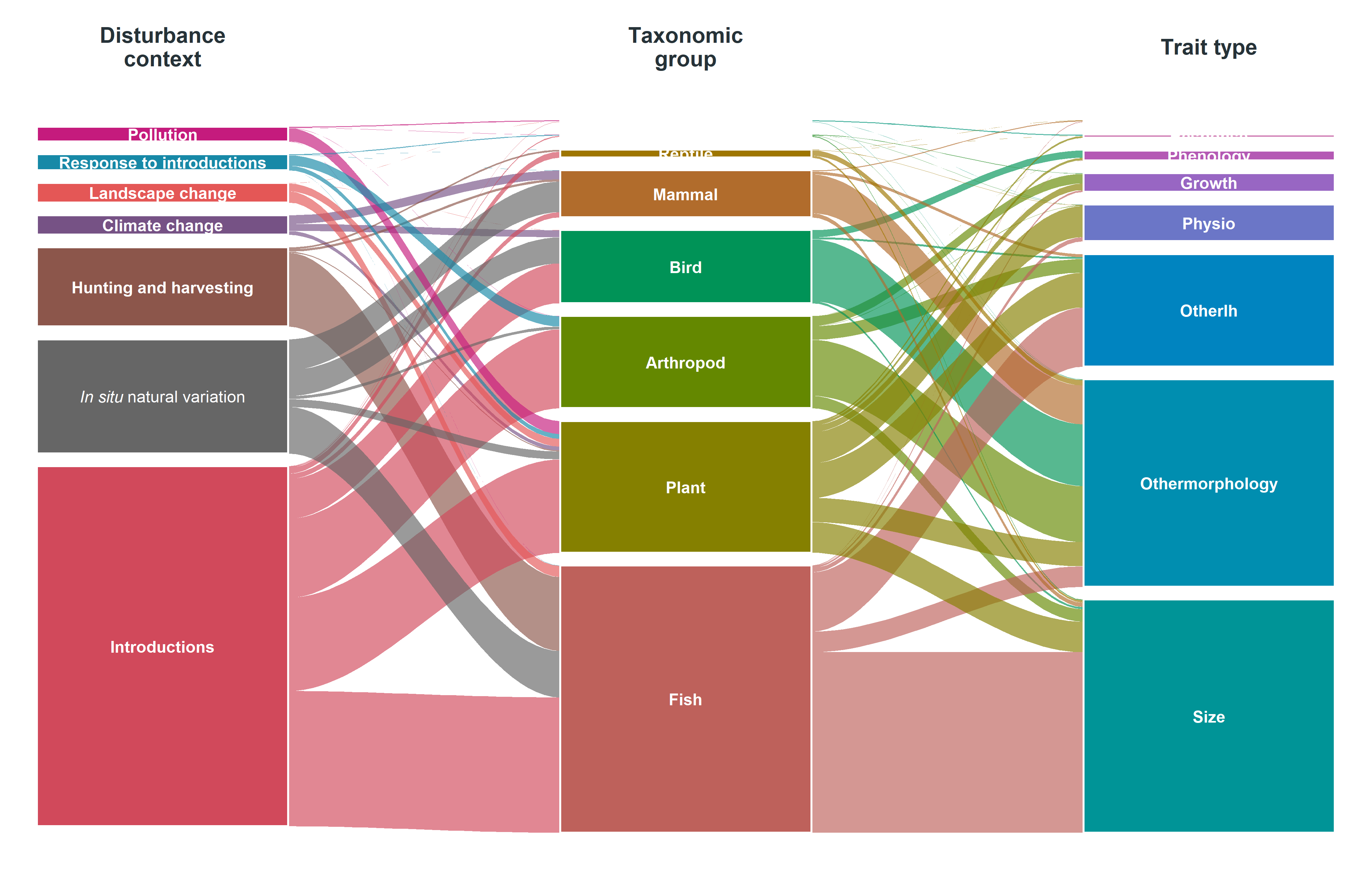
The second flow view links disturbance context to taxonomic group and then to
trait type. The accompanying table reports the taxon--trait pathways within
each disturbance context, so percentages sum to 100% within every context.
```{r}
#| label: tbl-m00-disturbance-taxa-trait
#| tbl-cap: "Taxonomic and trait representation within each disturbance context in model m00. Percentages are the share of contrasts within each disturbance context."
disturbance_taxa_trait <- m00_dat |>
  dplyr::transmute(
    `Disturbance context` = dplyr::coalesce(
      as.character(disturbance), "Not reported"
    ),
    `Taxonomic group` = dplyr::coalesce(as.character(taxa), "Not reported"),
    `Trait type` = dplyr::coalesce(as.character(trait_type), "Not reported")
  ) |>
  dplyr::count(
    `Disturbance context`, `Taxonomic group`, `Trait type`,
    name = "Contrasts"
  ) |>
  dplyr::group_by(`Disturbance context`) |>
  dplyr::mutate(`Within-context (%)` = 100 * Contrasts / sum(Contrasts)) |>
  dplyr::ungroup()

readr::write_csv(
  disturbance_taxa_trait,
  here::here("Rdata", "tables", "m00_disturbance_taxa_trait_percent.csv")
)

disturbance_taxa_trait |>
  dplyr::arrange(
    `Disturbance context`, dplyr::desc(`Within-context (%)`),
    `Taxonomic group`, `Trait type`
  ) |>
  dplyr::mutate(
    Contrasts = scales::comma(Contrasts),
    `Within-context (%)` = sprintf("%.1f", `Within-context (%)`)
  ) |>
  knitr::kable(align = c("l", "l", "l", "r", "r")) |>
  kableExtra::kable_styling(
    bootstrap_options = c("striped", "hover", "condensed", "responsive"),
    full_width = TRUE
  )
```
```{r}
#| label: fig-m00-alluvial-disturbance-taxa-trait
#| fig-cap: "Disturbance context, taxonomic representation, and trait type among the 7,186 contrasts retained by model m00. Flow width is proportional to the number of contrasts."
#| fig-alt: "An alluvial plot linking disturbance contexts to taxonomic groups and then trait types, with wider flows indicating more contrasts."
#| fig-width: 14
#| fig-height: 9
p_disturbance_taxa_trait <- make_alluvial(
  m00_dat,
  axes = c("disturbance", "taxa", "trait_type"),
  axis_labels = c(
    "Disturbance\ncontext", "Taxonomic\ngroup", "Trait type"
  )
)

ggplot2::ggsave(
  here::here("Rdata", "figures", "m00_alluvial_disturbance_taxa_trait.png"),
  p_disturbance_taxa_trait, width = 14, height = 9, dpi = 320, bg = "white"
)
ggplot2::ggsave(
  here::here("Figures", "m00_alluvial_disturbance_taxa_trait.pdf"),
  p_disturbance_taxa_trait, width = 14, height = 9,
  device = grDevices::cairo_pdf, bg = "white"
)

p_disturbance_taxa_trait
```
```{r pathway-summary}
pct_m00 <- function(x) sprintf("%.1f%%", 100 * mean(x, na.rm = TRUE))
m00_pathways <- m00_dat |>
  dplyr::count(disturbance, design, genphen, trait_type, sort = TRUE)
top_pathway <- m00_pathways[1, ]
```
Introductions contributed
`r pct_m00(m00_dat$disturbance == "Introduction")` of contrasts, and most contrasts were synchronic (`r pct_m00(m00_dat$design == "Synchronic")`)
and phenotypic (`r pct_m00(m00_dat$genphen == "Phenotypic")`). Size and
other-morphology traits together accounted for
`r pct_m00(m00_dat$trait_type %in% c("size", "othermorphology"))` of the
analytical sample. The largest single pathway was allochronic, phenotypic size
evidence under hunting or harvesting (`r top_pathway$n` contrasts;
`r sprintf("%.1f%%", 100 * top_pathway$n / nrow(m00_dat))`). The next four largest
pathways all arose from synchronic comparisons of introduced systems.
```{r by-genphen}
m00_dat |> dplyr::count(genphen, sort = TRUE)
```
```{r by-env-change}
m00_dat |> dplyr::count(env_change, sort = TRUE)
```
```{r by-data-type}
m00_dat |> dplyr::count(data_type, sort = TRUE)
```
```{r by-transf-data}
m00_dat |> dplyr::count(transf_data, sort = TRUE)
```
```{r by-data-scale}
m00_dat |> dplyr::count(data_scale, sort = TRUE)
```
## Donut summaries
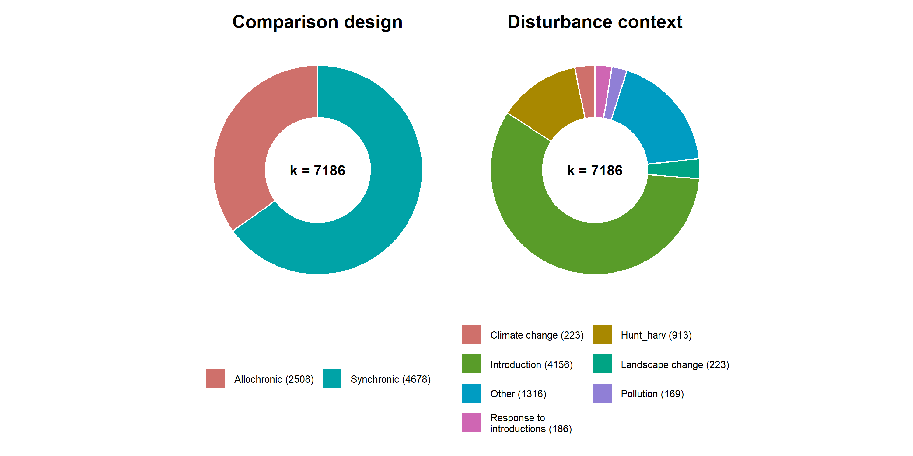
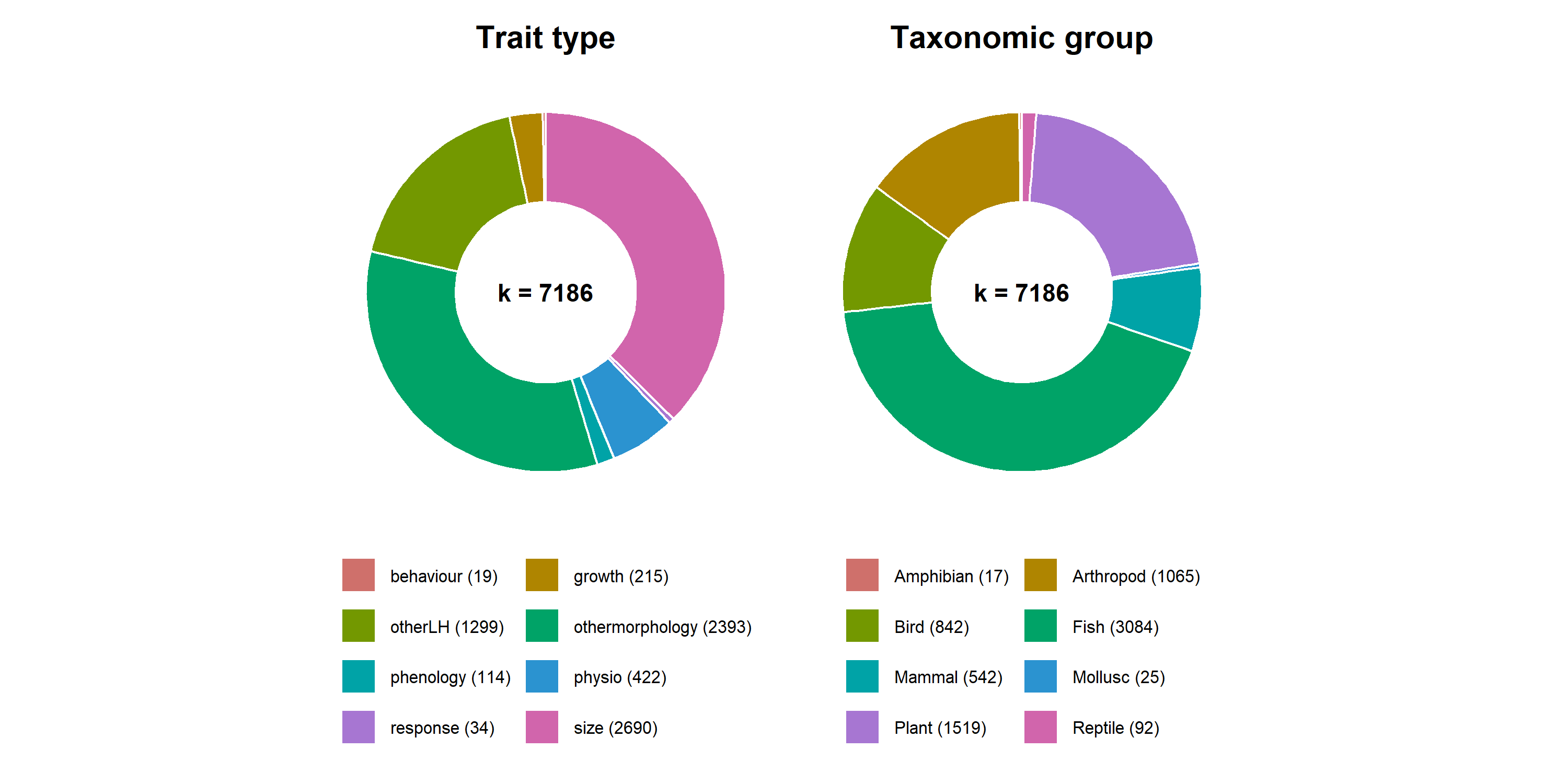
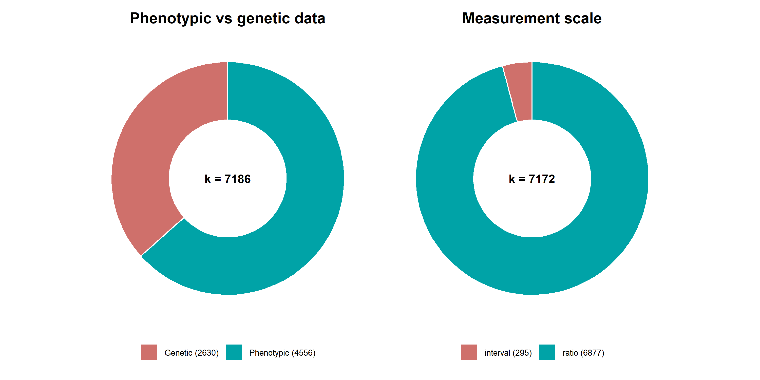
Each donut counts the `r scales::comma(nrow(m00_dat))` analysed contrasts.
```{r donut-design-disturbance, fig.width=10, fig.height=5}
plot_count_donut(m00_dat, "design", "Comparison design") +
  plot_count_donut(m00_dat, "disturbance", "Disturbance context") +
  patchwork::plot_layout(guides = "keep") &
  ggplot2::theme(legend.position = "bottom", legend.text = ggplot2::element_text(size = 8))
```
```{r donut-trait-taxa, fig.width=10, fig.height=5}
plot_count_donut(m00_dat, "trait_type", "Trait type") +
  plot_count_donut(m00_dat, "taxa", "Taxonomic group") +
  patchwork::plot_layout(guides = "keep") &
  ggplot2::theme(legend.position = "bottom", legend.text = ggplot2::element_text(size = 8))
```
```{r donut-data, fig.width=10, fig.height=5}
plot_count_donut(m00_dat, "genphen", "Phenotypic vs genetic data") +
  plot_count_donut(m00_dat, "data_scale", "Measurement scale") +
  patchwork::plot_layout(guides = "keep") &
  ggplot2::theme(legend.position = "bottom", legend.text = ggplot2::element_text(size = 8))
```
## Distributions
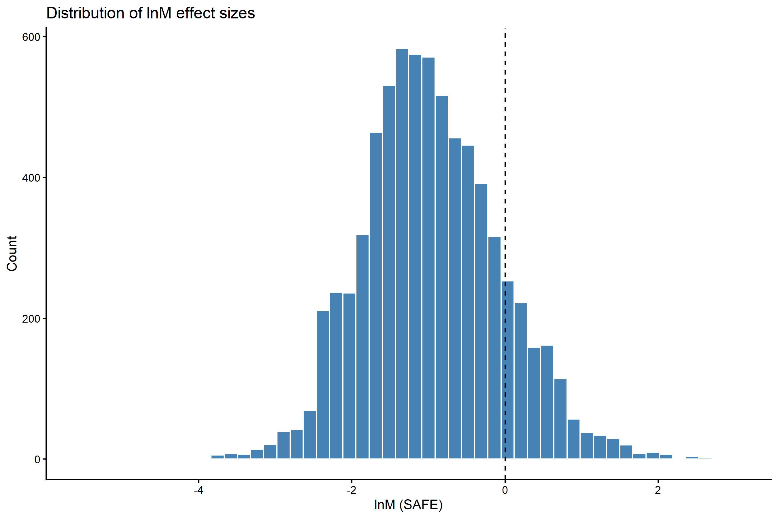
### lnM estimates
```{r dist-yi}
ggplot2::ggplot(m00_dat, ggplot2::aes(x = yi_lnM_safe)) +
  ggplot2::geom_histogram(bins = 50, fill = "steelblue", colour = "white") +
  ggplot2::geom_vline(xintercept = 0, linetype = "dashed") +
  ggplot2::labs(x = "lnM (SAFE)", y = "Count",
                title = "Distribution of lnM effect sizes") +
  ggplot2::theme_classic()
```
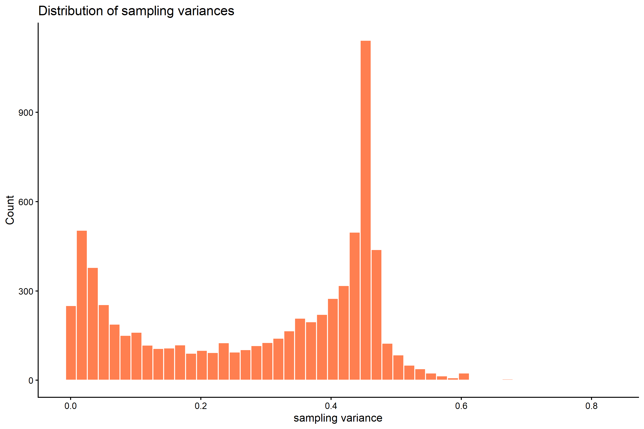
### Sampling variances
```{r dist-vi}
ggplot2::ggplot(m00_dat, ggplot2::aes(x = (vi_lnM_safe))) +
  ggplot2::geom_histogram(bins = 50, fill = "coral", colour = "white") +
  ggplot2::labs(x = "sampling variance", y = "Count",
                title = "Distribution of sampling variances") +
  ggplot2::theme_classic()
```
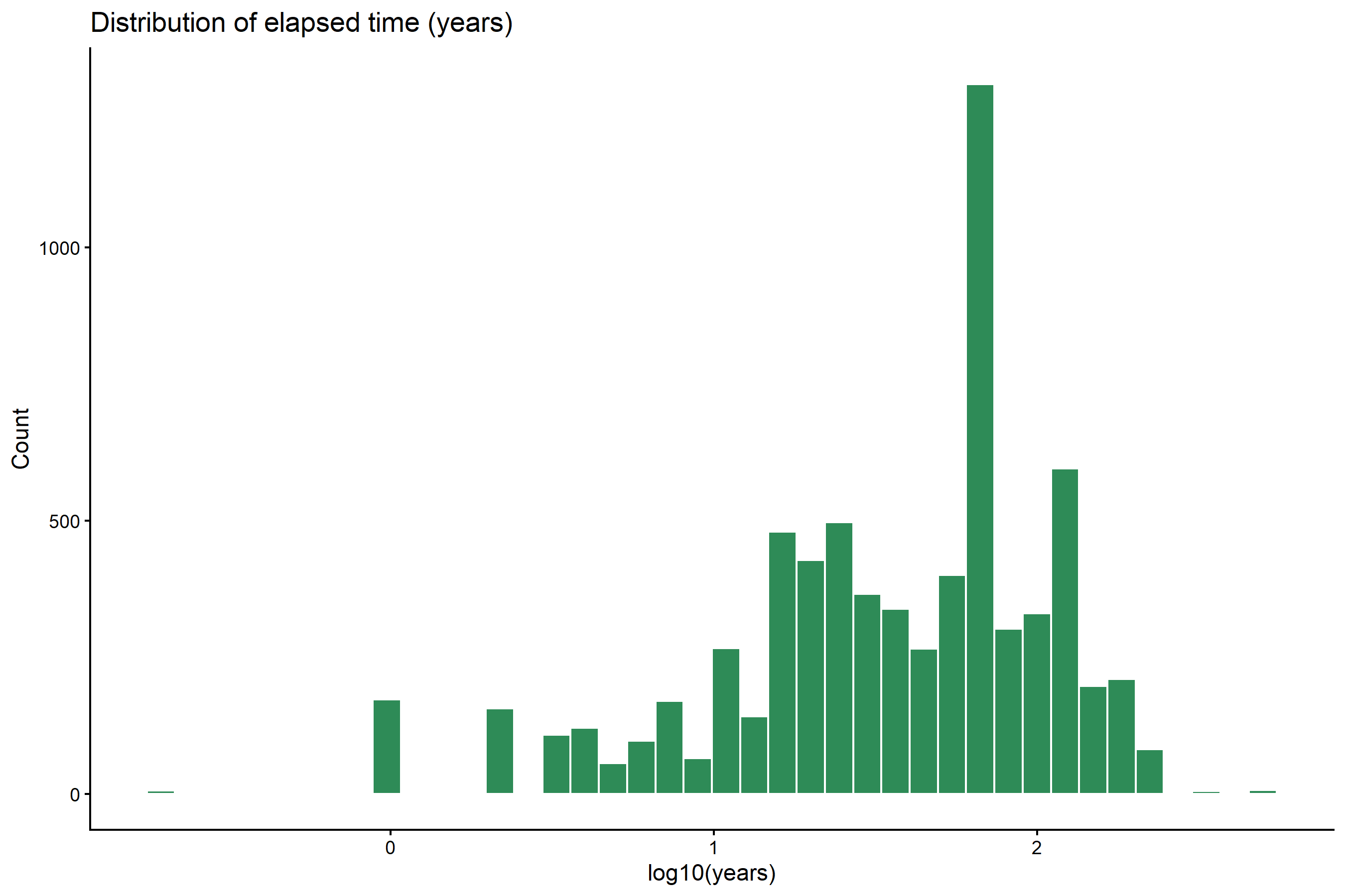
### Elapsed years
```{r dist-years}
m00_dat |>
  dplyr::filter(!is.na(log10_years)) |>
  ggplot2::ggplot(ggplot2::aes(x = log10_years)) +
  ggplot2::geom_histogram(bins = 40, fill = "seagreen", colour = "white") +
  ggplot2::labs(x = "log10(years)", y = "Count",
                title = "Distribution of elapsed time (years)") +
  ggplot2::theme_classic()
```
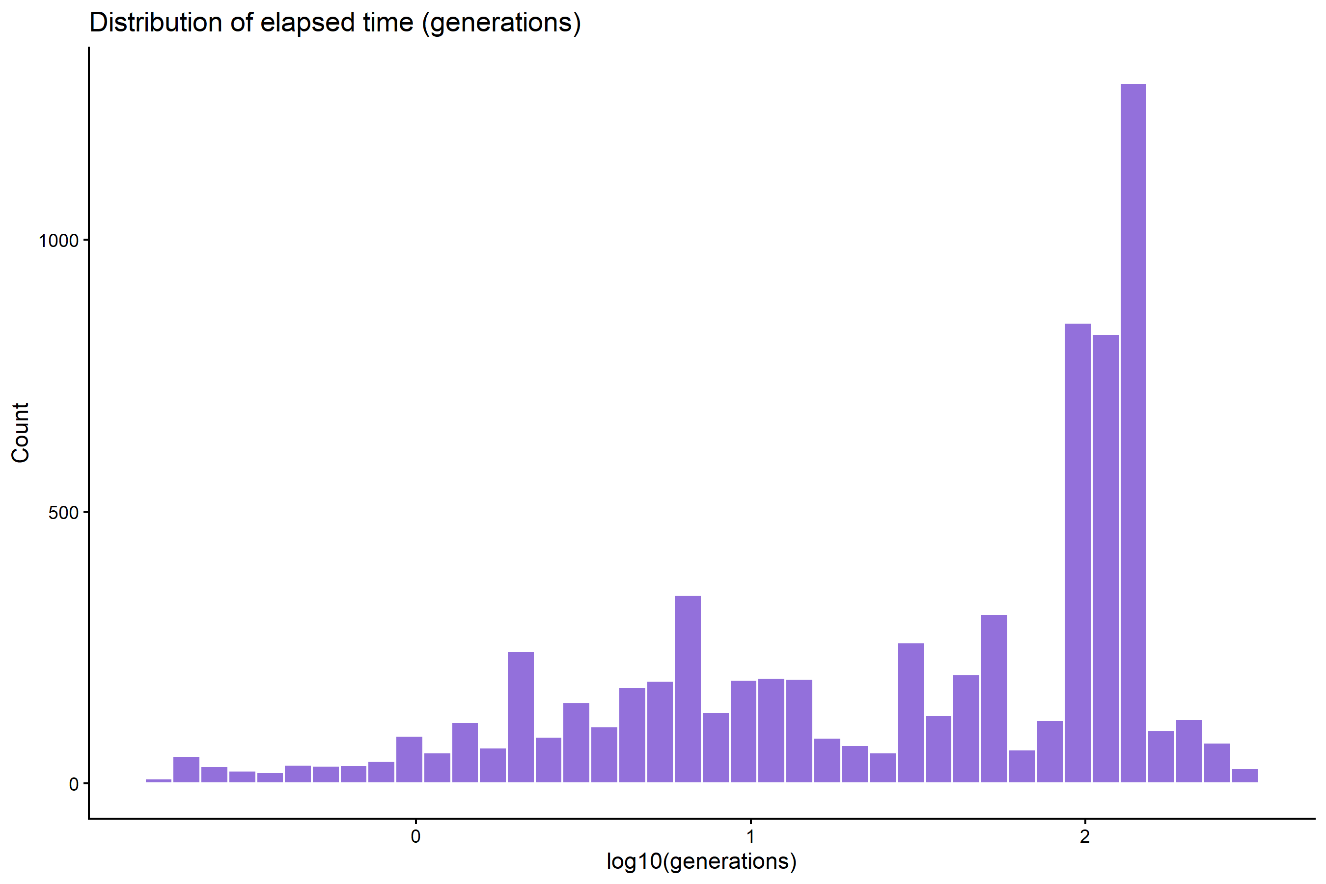
### Elapsed generations
```{r dist-gen}
m00_dat |>
  dplyr::filter(!is.na(log10_generations)) |>
  ggplot2::ggplot(ggplot2::aes(x = log10_generations)) +
  ggplot2::geom_histogram(bins = 40, fill = "mediumpurple", colour = "white") +
  ggplot2::labs(x = "log10(generations)", y = "Count",
                title = "Distribution of elapsed time (generations)") +
  ggplot2::theme_classic()
```
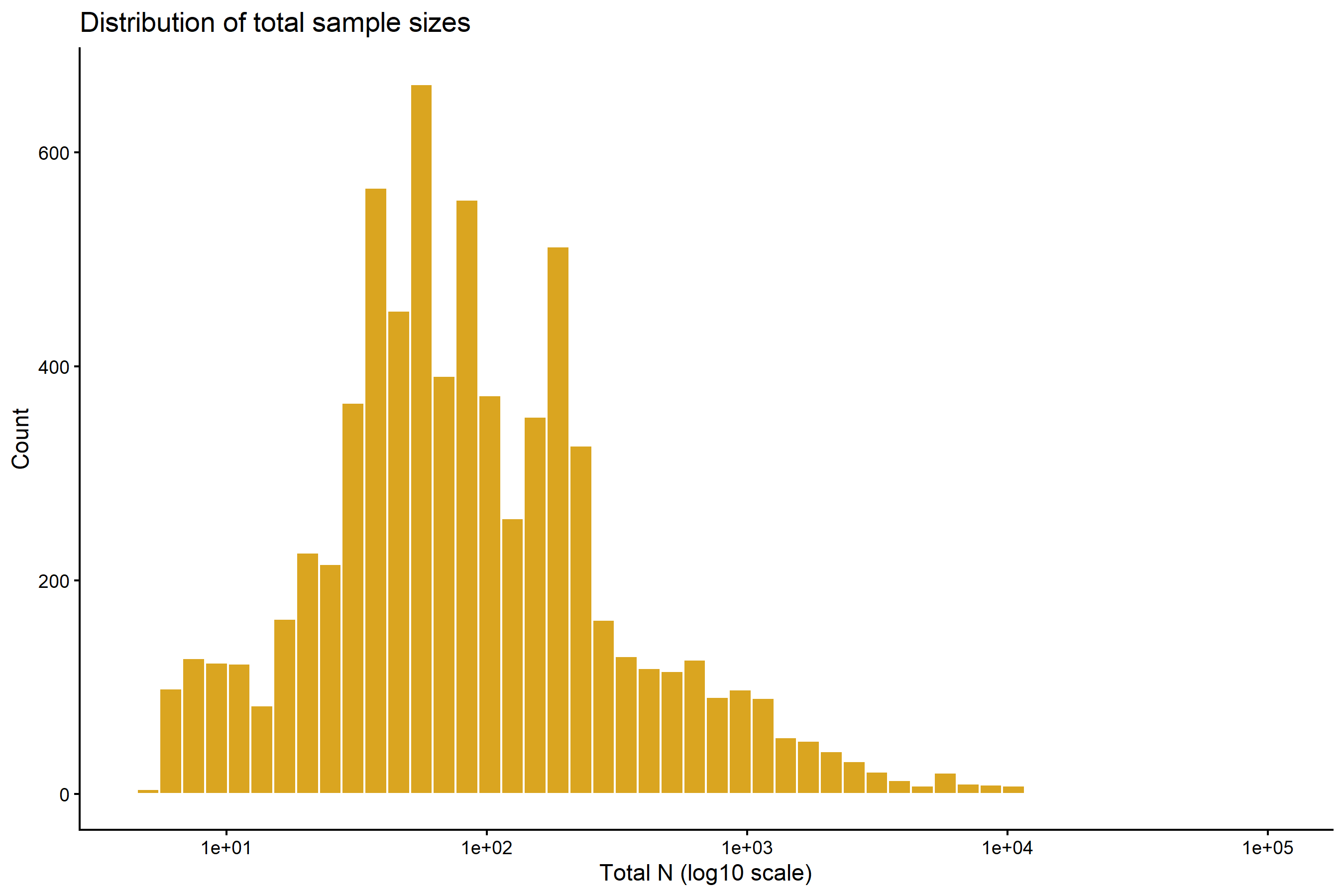
### Sample sizes
```{r dist-n}
m00_dat |>
  dplyr::filter(!is.na(n_total)) |>
  ggplot2::ggplot(ggplot2::aes(x = n_total)) +
  ggplot2::geom_histogram(bins = 50, fill = "goldenrod", colour = "white") +
  ggplot2::scale_x_log10() +
  ggplot2::labs(x = "Total N (log10 scale)", y = "Count",
                title = "Distribution of total sample sizes") +
  ggplot2::theme_classic()
```
## Save descriptive tables
```{r save-tables}
tab_overview <- m00_dat |>
  dplyr::summarise(
    k_contrasts   = dplyr::n(),
    n_studies     = dplyr::n_distinct(ref_id),
    n_systems     = dplyr::n_distinct(sys_id),
    n_species     = dplyr::n_distinct(canonical_lookup[as.character(sp_ncbi)]),
    n_allochronic = sum(design == "Allochronic", na.rm = TRUE),
    n_synchronic  = sum(design == "Synchronic",  na.rm = TRUE)
  )

readr::write_csv(tab_overview,
                 here::here("Rdata", "tables", "descriptive_overview.csv"))

for (var in c("disturbance", "design", "trait_type", "taxa",
               "genphen", "env_change", "data_type", "transf_data", "data_scale")) {
  tbl <- m00_dat |> dplyr::count(.data[[var]], sort = TRUE)
  readr::write_csv(
    tbl,
    here::here("Rdata", "tables", paste0("counts_by_", var, ".csv"))
  )
}

cat("Descriptive tables saved to Rdata/tables/\n")
```