Appendix E — Protocol deviation — moderators adjusted for elapsed time

E.1 Recorded change

This chapter was not part of the pre-registered protocol. It refits the primary moderators (disturbance, design, trait_type, genphen) with elapsed time added as an additive covariate.

NoteWhat changed—and what did not

Changed: for each of the four primary moderators, we fitted an additive location-scale model that adds elapsed time (log10_years, and separately log10_generations) as a second main-effect term, with no interaction. This adjusts each moderator’s estimate for the average elapsed-time difference between its levels, without letting the time slope itself vary by level.

Unchanged: the dataset, the moderator definitions, the ref_id and phylogenetic random effects, the priors, and the MCMC settings all match the primary single-moderator models.

This produces eight models: four moderators × two elapsed-time scales.

E.2 Moderator–time relationships

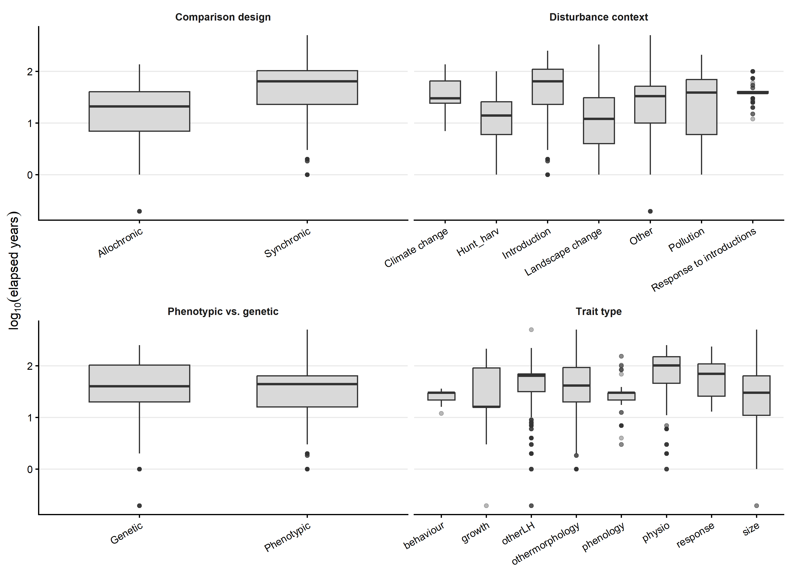
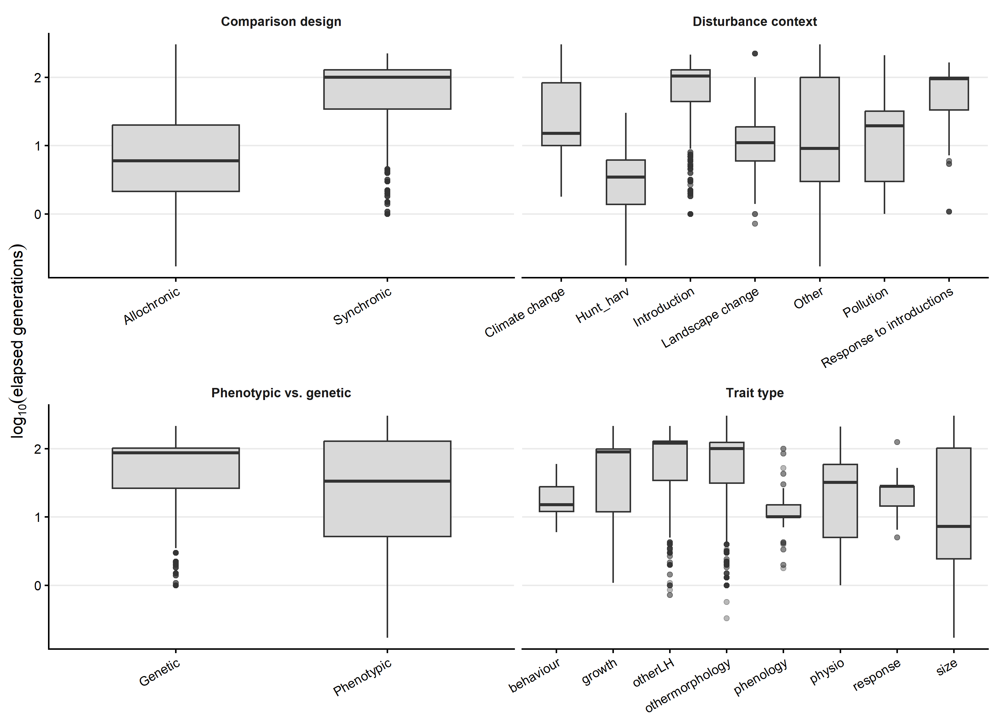
The plots below show how elapsed time is distributed across the levels of each moderator.

Code
source(here::here("Scripts", "00_packages.R"))

dat_es <- readRDS(here::here("Rdata", "effect_sizes", "proceed_lnm_safe.rds"))

moderator_labels <- c(
  disturbance = "Disturbance context",
  design      = "Comparison design",
  trait_type  = "Trait type",
  genphen     = "Phenotypic vs. genetic"
)

theme_deviation <- function(base_size = 13) {
  ggplot2::theme_classic(base_size = base_size) +
    ggplot2::theme(
      strip.background = ggplot2::element_blank(),
      strip.text        = ggplot2::element_text(face = "bold"),
      axis.text.x       = ggplot2::element_text(angle = 30, hjust = 1),
      panel.grid.major.y = ggplot2::element_line(colour = "grey92"),
      plot.title        = ggplot2::element_text(face = "bold")
    )
}

make_time_panel <- function(dat, timevar, timelabel) {
  long_dat <- purrr::map_dfr(names(moderator_labels), function(m) {
    dat |>
      dplyr::filter(!is.na(.data[[m]]), !is.na(.data[[timevar]])) |>
      dplyr::transmute(
        moderator_label = moderator_labels[[m]],
        level = as.character(.data[[m]]),
        time_value = .data[[timevar]]
      )
  })

  ggplot2::ggplot(long_dat, ggplot2::aes(x = level, y = time_value)) +
    ggplot2::geom_boxplot(fill = "grey85", outlier.alpha = 0.35, width = 0.6) +
    ggplot2::facet_wrap(~moderator_label, scales = "free_x", nrow = 2) +
    ggplot2::labs(x = NULL, y = timelabel) +
    theme_deviation()
}
Code
make_time_panel(dat_es, "log10_years", expression(log[10]("elapsed years")))

Elapsed years (log10 scale) across the levels of each primary moderator.
Code
make_time_panel(dat_es, "log10_generations", expression(log[10]("elapsed generations")))

Elapsed generations (log10 scale) across the levels of each primary moderator.

E.3 Model specification

Models were fitted on a remote server, not while rendering this book, using the same priors and MCMC settings as the primary models: 4 chains × 4,000 iterations (2,000 warmup), adapt_delta = 0.97, max_treedepth = 15, cmdstanr backend.

Code
loc_formula <- as.formula(paste0(
  "yi_lnM_safe ~ ", moderator, " + ", timevar,
  " + (1 | ref_id) + (1 | gr(sp_ncbi_canonical, cov = A))",
  " + (1 | gr(es_id_model, cov = V))"
))
scl_formula <- as.formula(paste0("sigma ~ ", moderator, " + ", timevar))

formula_add <- brms::bf(loc_formula, scl_formula)
fit_add <- brms::brm(
  formula = formula_add, data = dat_model, data2 = list(A = A_mod, V = V),
  prior = priors_add, chains = 4, iter = 4000, warmup = 2000, cores = 4,
  backend = "cmdstanr", control = list(adapt_delta = 0.97, max_treedepth = 15)
)

E.4 Convergence diagnostics

Code
diag_tbl <- readr::read_csv(
  here::here("Rdata", "tables", "additive_diagnostics.csv"),
  show_col_types = FALSE
)
knitr::kable(
  diag_tbl,
  col.names = c("Model", "Moderator", "Elapsed-time variable", "Max Rhat",
               "Min Bulk ESS", "Min Tail ESS", "Divergent transitions",
               "Max-treedepth hits"),
  digits = 3,
  caption = "Convergence diagnostics for the eight additive (moderator + time) models."
)
Convergence diagnostics for the eight additive (moderator + time) models.
Model Moderator Elapsed-time variable Max Rhat Min Bulk ESS Min Tail ESS Divergent transitions Max-treedepth hits
disturbance_plus_log10_years disturbance log10_years 1.040 110.422 85.168 10 0
disturbance_plus_log10_generations disturbance log10_generations 1.049 83.722 36.600 35 0
design_plus_log10_years design log10_years 1.004 1957.105 3304.621 0 0
design_plus_log10_generations design log10_generations 1.004 1708.873 3037.805 0 0
trait_type_plus_log10_years trait_type log10_years 1.014 266.470 224.024 0 0
trait_type_plus_log10_generations trait_type log10_generations 1.066 52.183 81.764 2 0
genphen_plus_log10_years genphen log10_years 1.005 1436.436 2809.353 0 0
genphen_plus_log10_generations genphen log10_generations 1.005 1276.362 2639.275 0 0

E.5 Model summaries

 Family: gaussian 
  Links: mu = identity; sigma = log 
Formula: yi_lnM_safe ~ disturbance + log10_years + (1 | ref_id) + (1 | gr(sp_ncbi_canonical, cov = A)) + (1 | gr(es_id_model, cov = V)) 
         sigma ~ disturbance + log10_years
   Data: dat_model (Number of observations: 7186) 
  Draws: 4 chains, each with iter = 4000; warmup = 2000; thin = 1;
         total post-warmup draws = 8000

Multilevel Hyperparameters:
~es_id_model (Number of levels: 7186) 
              Estimate Est.Error l-95% CI u-95% CI Rhat Bulk_ESS Tail_ESS
sd(Intercept)     1.00      0.00     1.00     1.00   NA       NA       NA

~ref_id (Number of levels: 254) 
              Estimate Est.Error l-95% CI u-95% CI Rhat Bulk_ESS Tail_ESS
sd(Intercept)     0.81      0.05     0.72     0.90 1.00     1839     3475

~sp_ncbi_canonical (Number of levels: 253) 
              Estimate Est.Error l-95% CI u-95% CI Rhat Bulk_ESS Tail_ESS
sd(Intercept)     0.82      0.13     0.60     1.10 1.01     1052     1969

Regression Coefficients:
                                         Estimate Est.Error l-95% CI u-95% CI
Intercept                                   -0.19      0.48    -1.11     0.76
sigma_Intercept                             -1.46      0.14    -1.76    -1.20
disturbanceHunt_harv                        -0.13      0.13    -0.39     0.13
disturbanceIntroduction                      0.06      0.16    -0.26     0.37
disturbanceLandscapechange                   0.11      0.19    -0.27     0.50
disturbanceOther                            -0.17      0.13    -0.44     0.08
disturbancePollution                         0.02      0.27    -0.51     0.54
disturbanceResponsetointroductions           0.02      0.26    -0.49     0.53
log10_years                                  0.07      0.02     0.02     0.12
sigma_disturbanceHunt_harv                   0.65      0.14     0.40     0.94
sigma_disturbanceIntroduction                0.22      0.13    -0.03     0.50
sigma_disturbanceLandscapechange            -1.07      0.37    -2.04    -0.50
sigma_disturbanceOther                       0.32      0.14     0.08     0.60
sigma_disturbancePollution                   0.15      0.21    -0.29     0.54
sigma_disturbanceResponsetointroductions     0.50      0.15     0.21     0.81
sigma_log10_years                            0.01      0.03    -0.05     0.08
                                         Rhat Bulk_ESS Tail_ESS
Intercept                                1.00     2065     3343
sigma_Intercept                          1.00      734     1112
disturbanceHunt_harv                     1.00     1470     2611
disturbanceIntroduction                  1.00     1453     2387
disturbanceLandscapechange               1.00     1475     2471
disturbanceOther                         1.00     1415     2457
disturbancePollution                     1.00     1816     3099
disturbanceResponsetointroductions       1.00     1774     3323
log10_years                              1.00     3715     5906
sigma_disturbanceHunt_harv               1.00      704     1144
sigma_disturbanceIntroduction            1.00      676     1137
sigma_disturbanceLandscapechange         1.04      110       85
sigma_disturbanceOther                   1.00      728     1126
sigma_disturbancePollution               1.00      744     1253
sigma_disturbanceResponsetointroductions 1.00      827     1490
sigma_log10_years                        1.00     2178     4061

Draws were sampled using sample(hmc). For each parameter, Bulk_ESS
and Tail_ESS are effective sample size measures, and Rhat is the potential
scale reduction factor on split chains (at convergence, Rhat = 1).
 Family: gaussian 
  Links: mu = identity; sigma = log 
Formula: yi_lnM_safe ~ disturbance + log10_generations + (1 | ref_id) + (1 | gr(sp_ncbi_canonical, cov = A)) + (1 | gr(es_id_model, cov = V)) 
         sigma ~ disturbance + log10_generations
   Data: dat_model (Number of observations: 7186) 
  Draws: 4 chains, each with iter = 4000; warmup = 2000; thin = 1;
         total post-warmup draws = 8000

Multilevel Hyperparameters:
~es_id_model (Number of levels: 7186) 
              Estimate Est.Error l-95% CI u-95% CI Rhat Bulk_ESS Tail_ESS
sd(Intercept)     1.00      0.00     1.00     1.00   NA       NA       NA

~ref_id (Number of levels: 254) 
              Estimate Est.Error l-95% CI u-95% CI Rhat Bulk_ESS Tail_ESS
sd(Intercept)     0.80      0.05     0.72     0.90 1.00     2356     4305

~sp_ncbi_canonical (Number of levels: 253) 
              Estimate Est.Error l-95% CI u-95% CI Rhat Bulk_ESS Tail_ESS
sd(Intercept)     0.86      0.13     0.63     1.12 1.00     1329     3104

Regression Coefficients:
                                         Estimate Est.Error l-95% CI u-95% CI
Intercept                                   -0.18      0.47    -1.12     0.74
sigma_Intercept                             -1.14      0.14    -1.44    -0.88
disturbanceHunt_harv                        -0.12      0.12    -0.36     0.13
disturbanceIntroduction                      0.03      0.16    -0.27     0.34
disturbanceLandscapechange                   0.12      0.19    -0.24     0.49
disturbanceOther                            -0.17      0.12    -0.41     0.07
disturbancePollution                         0.01      0.27    -0.51     0.54
disturbanceResponsetointroductions           0.01      0.26    -0.49     0.52
log10_generations                            0.09      0.03     0.04     0.14
sigma_disturbanceHunt_harv                   0.43      0.14     0.17     0.73
sigma_disturbanceIntroduction                0.32      0.14     0.07     0.62
sigma_disturbanceLandscapechange            -1.30      0.42    -2.26    -0.60
sigma_disturbanceOther                       0.19      0.14    -0.07     0.48
sigma_disturbancePollution                   0.08      0.22    -0.36     0.49
sigma_disturbanceResponsetointroductions     0.53      0.16     0.23     0.84
sigma_log10_generations                     -0.22      0.03    -0.27    -0.16
                                         Rhat Bulk_ESS Tail_ESS
Intercept                                1.00     2700     3593
sigma_Intercept                          1.01      612     1193
disturbanceHunt_harv                     1.00     1691     3056
disturbanceIntroduction                  1.00     1609     3050
disturbanceLandscapechange               1.00     1844     3149
disturbanceOther                         1.00     1639     3188
disturbancePollution                     1.00     2269     3279
disturbanceResponsetointroductions       1.00     2544     4024
log10_generations                        1.00     4925     5951
sigma_disturbanceHunt_harv               1.01      637     1174
sigma_disturbanceIntroduction            1.01      614     1111
sigma_disturbanceLandscapechange         1.05       85       37
sigma_disturbanceOther                   1.01      641     1234
sigma_disturbancePollution               1.00      667     1515
sigma_disturbanceResponsetointroductions 1.01      697     1329
sigma_log10_generations                  1.00     2584     4478

Draws were sampled using sample(hmc). For each parameter, Bulk_ESS
and Tail_ESS are effective sample size measures, and Rhat is the potential
scale reduction factor on split chains (at convergence, Rhat = 1).
 Family: gaussian 
  Links: mu = identity; sigma = log 
Formula: yi_lnM_safe ~ design + log10_years + (1 | ref_id) + (1 | gr(sp_ncbi_canonical, cov = A)) + (1 | gr(es_id_model, cov = V)) 
         sigma ~ design + log10_years
   Data: dat_model (Number of observations: 7186) 
  Draws: 4 chains, each with iter = 4000; warmup = 2000; thin = 1;
         total post-warmup draws = 8000

Multilevel Hyperparameters:
~es_id_model (Number of levels: 7186) 
              Estimate Est.Error l-95% CI u-95% CI Rhat Bulk_ESS Tail_ESS
sd(Intercept)     1.00      0.00     1.00     1.00   NA       NA       NA

~ref_id (Number of levels: 254) 
              Estimate Est.Error l-95% CI u-95% CI Rhat Bulk_ESS Tail_ESS
sd(Intercept)     0.80      0.05     0.72     0.89 1.00     3146     4656

~sp_ncbi_canonical (Number of levels: 253) 
              Estimate Est.Error l-95% CI u-95% CI Rhat Bulk_ESS Tail_ESS
sd(Intercept)     0.78      0.12     0.57     1.04 1.00     2309     4313

Regression Coefficients:
                       Estimate Est.Error l-95% CI u-95% CI Rhat Bulk_ESS
Intercept                 -0.33      0.42    -1.16     0.50 1.00     5057
sigma_Intercept           -0.96      0.04    -1.04    -0.87 1.00     3397
designSynchronic           0.21      0.07     0.08     0.35 1.00     6786
log10_years                0.07      0.02     0.03     0.12 1.00    11088
sigma_designSynchronic    -0.23      0.03    -0.30    -0.16 1.00     3061
sigma_log10_years         -0.01      0.03    -0.08     0.06 1.00     2713
                       Tail_ESS
Intercept                  5140
sigma_Intercept            5603
designSynchronic           6418
log10_years                6732
sigma_designSynchronic     5562
sigma_log10_years          5552

Draws were sampled using sample(hmc). For each parameter, Bulk_ESS
and Tail_ESS are effective sample size measures, and Rhat is the potential
scale reduction factor on split chains (at convergence, Rhat = 1).
 Family: gaussian 
  Links: mu = identity; sigma = log 
Formula: yi_lnM_safe ~ design + log10_generations + (1 | ref_id) + (1 | gr(sp_ncbi_canonical, cov = A)) + (1 | gr(es_id_model, cov = V)) 
         sigma ~ design + log10_generations
   Data: dat_model (Number of observations: 7186) 
  Draws: 4 chains, each with iter = 4000; warmup = 2000; thin = 1;
         total post-warmup draws = 8000

Multilevel Hyperparameters:
~es_id_model (Number of levels: 7186) 
              Estimate Est.Error l-95% CI u-95% CI Rhat Bulk_ESS Tail_ESS
sd(Intercept)     1.00      0.00     1.00     1.00   NA       NA       NA

~ref_id (Number of levels: 254) 
              Estimate Est.Error l-95% CI u-95% CI Rhat Bulk_ESS Tail_ESS
sd(Intercept)     0.79      0.04     0.71     0.88 1.00     2974     4901

~sp_ncbi_canonical (Number of levels: 253) 
              Estimate Est.Error l-95% CI u-95% CI Rhat Bulk_ESS Tail_ESS
sd(Intercept)     0.83      0.12     0.62     1.09 1.00     1878     3448

Regression Coefficients:
                        Estimate Est.Error l-95% CI u-95% CI Rhat Bulk_ESS
Intercept                  -0.33      0.46    -1.24     0.56 1.00     3540
sigma_Intercept            -0.82      0.03    -0.87    -0.77 1.00     5352
designSynchronic            0.18      0.07     0.04     0.31 1.00     4783
log10_generations           0.09      0.03     0.04     0.14 1.00     8432
sigma_designSynchronic      0.06      0.04    -0.02     0.14 1.00     2379
sigma_log10_generations    -0.25      0.03    -0.30    -0.20 1.00     2398
                        Tail_ESS
Intercept                   4541
sigma_Intercept             6453
designSynchronic            5512
log10_generations           6341
sigma_designSynchronic      4274
sigma_log10_generations     4084

Draws were sampled using sample(hmc). For each parameter, Bulk_ESS
and Tail_ESS are effective sample size measures, and Rhat is the potential
scale reduction factor on split chains (at convergence, Rhat = 1).
 Family: gaussian 
  Links: mu = identity; sigma = log 
Formula: yi_lnM_safe ~ trait_type + log10_years + (1 | ref_id) + (1 | gr(sp_ncbi_canonical, cov = A)) + (1 | gr(es_id_model, cov = V)) 
         sigma ~ trait_type + log10_years
   Data: dat_model (Number of observations: 7186) 
  Draws: 4 chains, each with iter = 4000; warmup = 2000; thin = 1;
         total post-warmup draws = 8000

Multilevel Hyperparameters:
~es_id_model (Number of levels: 7186) 
              Estimate Est.Error l-95% CI u-95% CI Rhat Bulk_ESS Tail_ESS
sd(Intercept)     1.00      0.00     1.00     1.00   NA       NA       NA

~ref_id (Number of levels: 254) 
              Estimate Est.Error l-95% CI u-95% CI Rhat Bulk_ESS Tail_ESS
sd(Intercept)     0.80      0.05     0.72     0.89 1.00     3305     4961

~sp_ncbi_canonical (Number of levels: 253) 
              Estimate Est.Error l-95% CI u-95% CI Rhat Bulk_ESS Tail_ESS
sd(Intercept)     0.81      0.11     0.61     1.06 1.00     2012     3831

Regression Coefficients:
                                Estimate Est.Error l-95% CI u-95% CI Rhat
Intercept                          -0.52      0.51    -1.54     0.49 1.00
sigma_Intercept                    -1.04      0.26    -1.58    -0.54 1.00
trait_typegrowth                    0.34      0.25    -0.14     0.83 1.00
trait_typeotherLH                   0.43      0.25    -0.04     0.91 1.00
trait_typeothermorphology           0.35      0.25    -0.12     0.84 1.00
trait_typephenology                 0.26      0.27    -0.26     0.78 1.00
trait_typephysio                    0.24      0.25    -0.22     0.73 1.00
trait_typeresponse                  0.47      0.27    -0.06     1.01 1.00
trait_typesize                      0.36      0.25    -0.11     0.84 1.00
log10_years                         0.08      0.02     0.04     0.13 1.00
sigma_trait_typegrowth             -1.15      0.40    -2.04    -0.44 1.01
sigma_trait_typeotherLH             0.18      0.26    -0.32     0.71 1.00
sigma_trait_typeothermorphology    -0.93      0.26    -1.43    -0.41 1.00
sigma_trait_typephenology           0.21      0.29    -0.35     0.79 1.00
sigma_trait_typephysio             -0.22      0.28    -0.76     0.31 1.00
sigma_trait_typeresponse            0.03      0.36    -0.68     0.70 1.00
sigma_trait_typesize                0.21      0.26    -0.29     0.73 1.00
sigma_log10_years                  -0.06      0.03    -0.11     0.00 1.00
                                Bulk_ESS Tail_ESS
Intercept                           3469     4643
sigma_Intercept                     1896     2985
trait_typegrowth                    2192     3870
trait_typeotherLH                   2194     3790
trait_typeothermorphology           2187     3954
trait_typephenology                 2393     3882
trait_typephysio                    2199     3810
trait_typeresponse                  2516     4573
trait_typesize                      2207     4027
log10_years                         7671     7136
sigma_trait_typegrowth               266      224
sigma_trait_typeotherLH             1903     3127
sigma_trait_typeothermorphology     1871     2889
sigma_trait_typephenology           1798     3130
sigma_trait_typephysio              1538     2948
sigma_trait_typeresponse            2052     3614
sigma_trait_typesize                1912     3115
sigma_log10_years                   3187     5182

Draws were sampled using sample(hmc). For each parameter, Bulk_ESS
and Tail_ESS are effective sample size measures, and Rhat is the potential
scale reduction factor on split chains (at convergence, Rhat = 1).
 Family: gaussian 
  Links: mu = identity; sigma = log 
Formula: yi_lnM_safe ~ trait_type + log10_generations + (1 | ref_id) + (1 | gr(sp_ncbi_canonical, cov = A)) + (1 | gr(es_id_model, cov = V)) 
         sigma ~ trait_type + log10_generations
   Data: dat_model (Number of observations: 7186) 
  Draws: 4 chains, each with iter = 4000; warmup = 2000; thin = 1;
         total post-warmup draws = 8000

Multilevel Hyperparameters:
~es_id_model (Number of levels: 7186) 
              Estimate Est.Error l-95% CI u-95% CI Rhat Bulk_ESS Tail_ESS
sd(Intercept)     1.00      0.00     1.00     1.00   NA       NA       NA

~ref_id (Number of levels: 254) 
              Estimate Est.Error l-95% CI u-95% CI Rhat Bulk_ESS Tail_ESS
sd(Intercept)     0.79      0.05     0.71     0.89 1.00     3608     4495

~sp_ncbi_canonical (Number of levels: 253) 
              Estimate Est.Error l-95% CI u-95% CI Rhat Bulk_ESS Tail_ESS
sd(Intercept)     0.83      0.12     0.62     1.08 1.00     2083     4012

Regression Coefficients:
                                Estimate Est.Error l-95% CI u-95% CI Rhat
Intercept                          -0.53      0.52    -1.54     0.48 1.00
sigma_Intercept                    -0.96      0.26    -1.48    -0.45 1.00
trait_typegrowth                    0.34      0.25    -0.15     0.83 1.00
trait_typeotherLH                   0.43      0.25    -0.06     0.92 1.00
trait_typeothermorphology           0.35      0.25    -0.14     0.84 1.00
trait_typephenology                 0.25      0.27    -0.29     0.79 1.00
trait_typephysio                    0.25      0.25    -0.24     0.74 1.00
trait_typeresponse                  0.48      0.28    -0.07     1.01 1.00
trait_typesize                      0.36      0.25    -0.13     0.85 1.00
log10_generations                   0.10      0.02     0.05     0.15 1.00
sigma_trait_typegrowth             -1.16      0.44    -2.19    -0.42 1.07
sigma_trait_typeotherLH             0.22      0.26    -0.30     0.74 1.00
sigma_trait_typeothermorphology    -0.88      0.26    -1.39    -0.36 1.00
sigma_trait_typephenology           0.19      0.29    -0.39     0.75 1.00
sigma_trait_typephysio             -0.23      0.28    -0.78     0.32 1.00
sigma_trait_typeresponse            0.03      0.35    -0.67     0.71 1.00
sigma_trait_typesize                0.16      0.26    -0.36     0.67 1.00
sigma_log10_generations            -0.12      0.02    -0.16    -0.08 1.00
                                Bulk_ESS Tail_ESS
Intercept                           4355     4686
sigma_Intercept                     1829     3128
trait_typegrowth                    2488     3329
trait_typeotherLH                   2506     3550
trait_typeothermorphology           2516     3243
trait_typephenology                 2774     4161
trait_typephysio                    2544     3348
trait_typeresponse                  2851     4436
trait_typesize                      2510     3443
log10_generations                   8633     6936
sigma_trait_typegrowth                52       82
sigma_trait_typeotherLH             1799     3020
sigma_trait_typeothermorphology     1816     3061
sigma_trait_typephenology           1953     3599
sigma_trait_typephysio              1570     2973
sigma_trait_typeresponse            2374     3853
sigma_trait_typesize                1827     3026
sigma_log10_generations             3048     5066

Draws were sampled using sample(hmc). For each parameter, Bulk_ESS
and Tail_ESS are effective sample size measures, and Rhat is the potential
scale reduction factor on split chains (at convergence, Rhat = 1).
 Family: gaussian 
  Links: mu = identity; sigma = log 
Formula: yi_lnM_safe ~ genphen + log10_years + (1 | ref_id) + (1 | gr(sp_ncbi_canonical, cov = A)) + (1 | gr(es_id_model, cov = V)) 
         sigma ~ genphen + log10_years
   Data: dat_model (Number of observations: 7186) 
  Draws: 4 chains, each with iter = 4000; warmup = 2000; thin = 1;
         total post-warmup draws = 8000

Multilevel Hyperparameters:
~es_id_model (Number of levels: 7186) 
              Estimate Est.Error l-95% CI u-95% CI Rhat Bulk_ESS Tail_ESS
sd(Intercept)     1.00      0.00     1.00     1.00   NA       NA       NA

~ref_id (Number of levels: 254) 
              Estimate Est.Error l-95% CI u-95% CI Rhat Bulk_ESS Tail_ESS
sd(Intercept)     0.81      0.05     0.72     0.90 1.00     2639     4821

~sp_ncbi_canonical (Number of levels: 253) 
              Estimate Est.Error l-95% CI u-95% CI Rhat Bulk_ESS Tail_ESS
sd(Intercept)     0.78      0.12     0.58     1.04 1.00     2097     3989

Regression Coefficients:
                        Estimate Est.Error l-95% CI u-95% CI Rhat Bulk_ESS
Intercept                  -0.17      0.44    -1.03     0.69 1.00     4016
sigma_Intercept            -1.30      0.05    -1.41    -1.20 1.00     2259
genphenPhenotypic          -0.07      0.05    -0.17     0.03 1.00     5692
log10_years                 0.08      0.03     0.03     0.13 1.00     8923
sigma_genphenPhenotypic     0.40      0.03     0.33     0.47 1.00     1962
sigma_log10_years          -0.07      0.03    -0.13    -0.02 1.00     3141
                        Tail_ESS
Intercept                   4886
sigma_Intercept             3929
genphenPhenotypic           5864
log10_years                 6492
sigma_genphenPhenotypic     3593
sigma_log10_years           4798

Draws were sampled using sample(hmc). For each parameter, Bulk_ESS
and Tail_ESS are effective sample size measures, and Rhat is the potential
scale reduction factor on split chains (at convergence, Rhat = 1).
 Family: gaussian 
  Links: mu = identity; sigma = log 
Formula: yi_lnM_safe ~ genphen + log10_generations + (1 | ref_id) + (1 | gr(sp_ncbi_canonical, cov = A)) + (1 | gr(es_id_model, cov = V)) 
         sigma ~ genphen + log10_generations
   Data: dat_model (Number of observations: 7186) 
  Draws: 4 chains, each with iter = 4000; warmup = 2000; thin = 1;
         total post-warmup draws = 8000

Multilevel Hyperparameters:
~es_id_model (Number of levels: 7186) 
              Estimate Est.Error l-95% CI u-95% CI Rhat Bulk_ESS Tail_ESS
sd(Intercept)     1.00      0.00     1.00     1.00   NA       NA       NA

~ref_id (Number of levels: 254) 
              Estimate Est.Error l-95% CI u-95% CI Rhat Bulk_ESS Tail_ESS
sd(Intercept)     0.80      0.05     0.71     0.89 1.00     3029     4567

~sp_ncbi_canonical (Number of levels: 253) 
              Estimate Est.Error l-95% CI u-95% CI Rhat Bulk_ESS Tail_ESS
sd(Intercept)     0.80      0.12     0.60     1.05 1.00     2234     3087

Regression Coefficients:
                        Estimate Est.Error l-95% CI u-95% CI Rhat Bulk_ESS
Intercept                  -0.19      0.44    -1.04     0.66 1.00     4031
sigma_Intercept            -1.13      0.04    -1.21    -1.05 1.00     2209
genphenPhenotypic          -0.06      0.05    -0.15     0.04 1.00     5633
log10_generations           0.10      0.03     0.05     0.15 1.00     8539
sigma_genphenPhenotypic     0.34      0.04     0.27     0.41 1.00     1849
sigma_log10_generations    -0.18      0.02    -0.22    -0.15 1.00     3851
                        Tail_ESS
Intercept                   5230
sigma_Intercept             4065
genphenPhenotypic           5602
log10_generations           7022
sigma_genphenPhenotypic     3283
sigma_log10_generations     5865

Draws were sampled using sample(hmc). For each parameter, Bulk_ESS
and Tail_ESS are effective sample size measures, and Rhat is the potential
scale reduction factor on split chains (at convergence, Rhat = 1).

E.6 Orchard-style figures

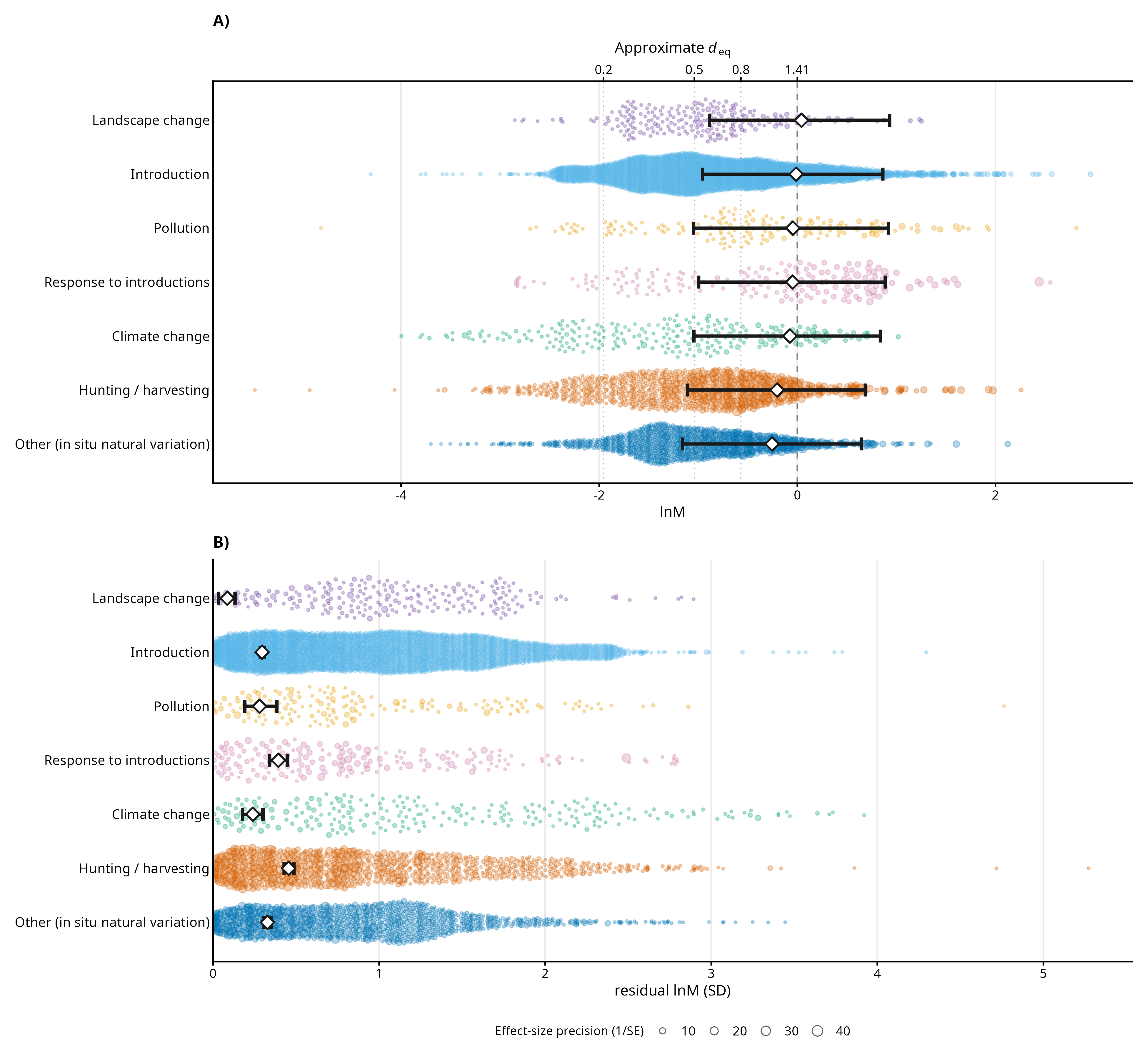
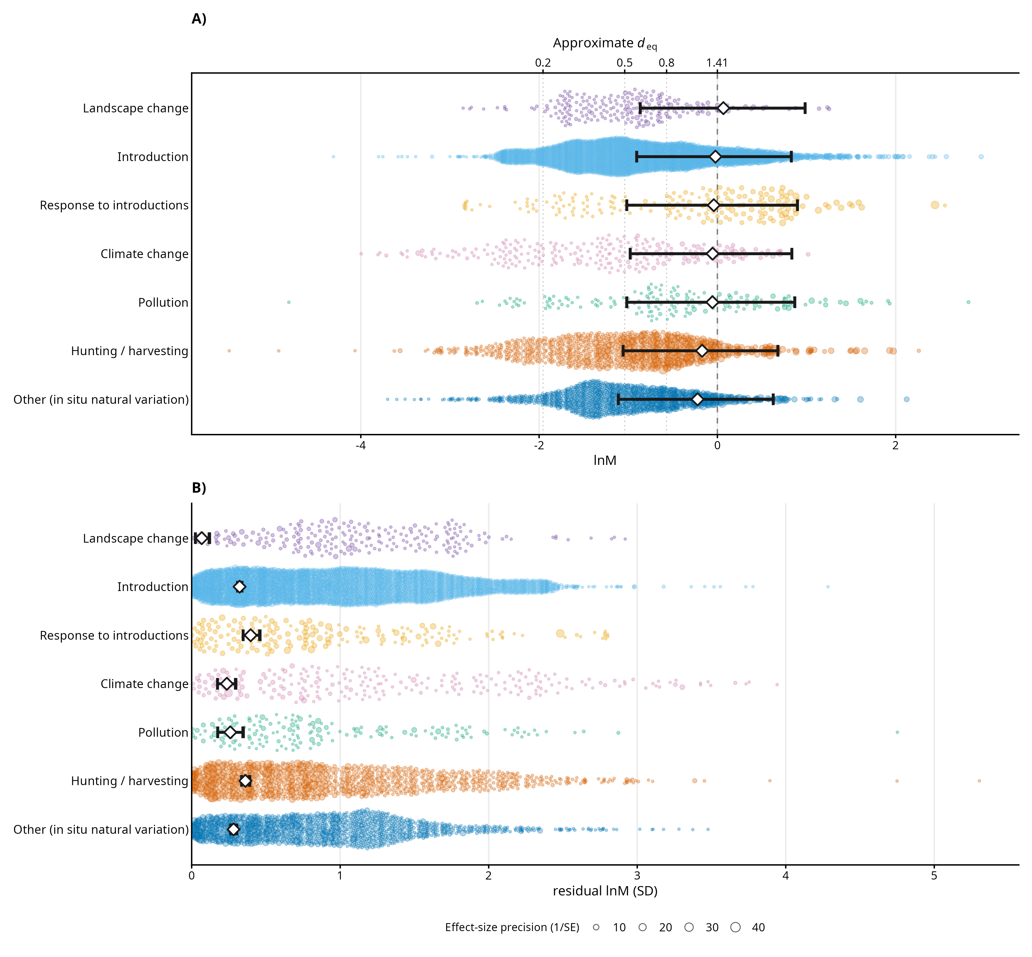
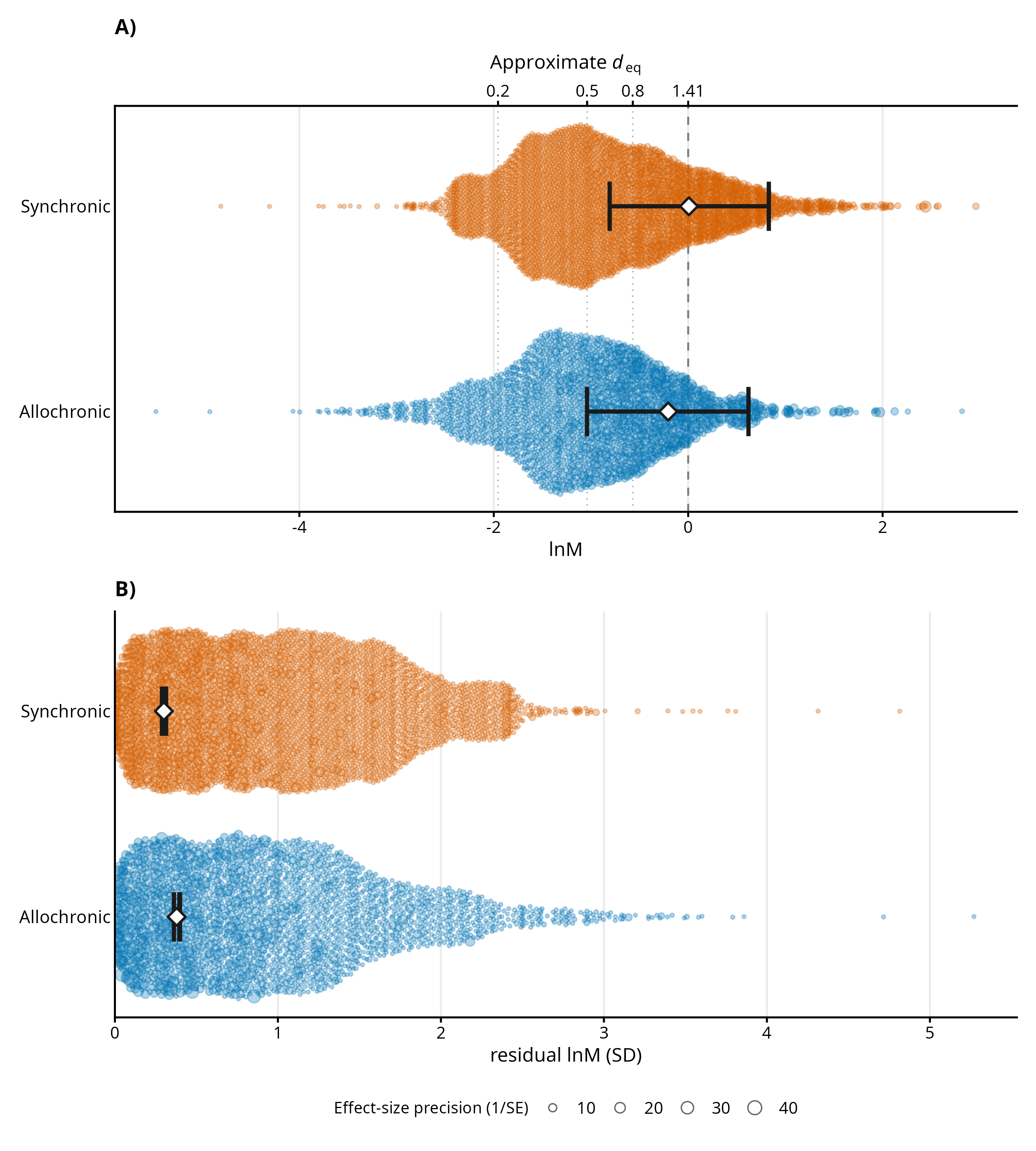
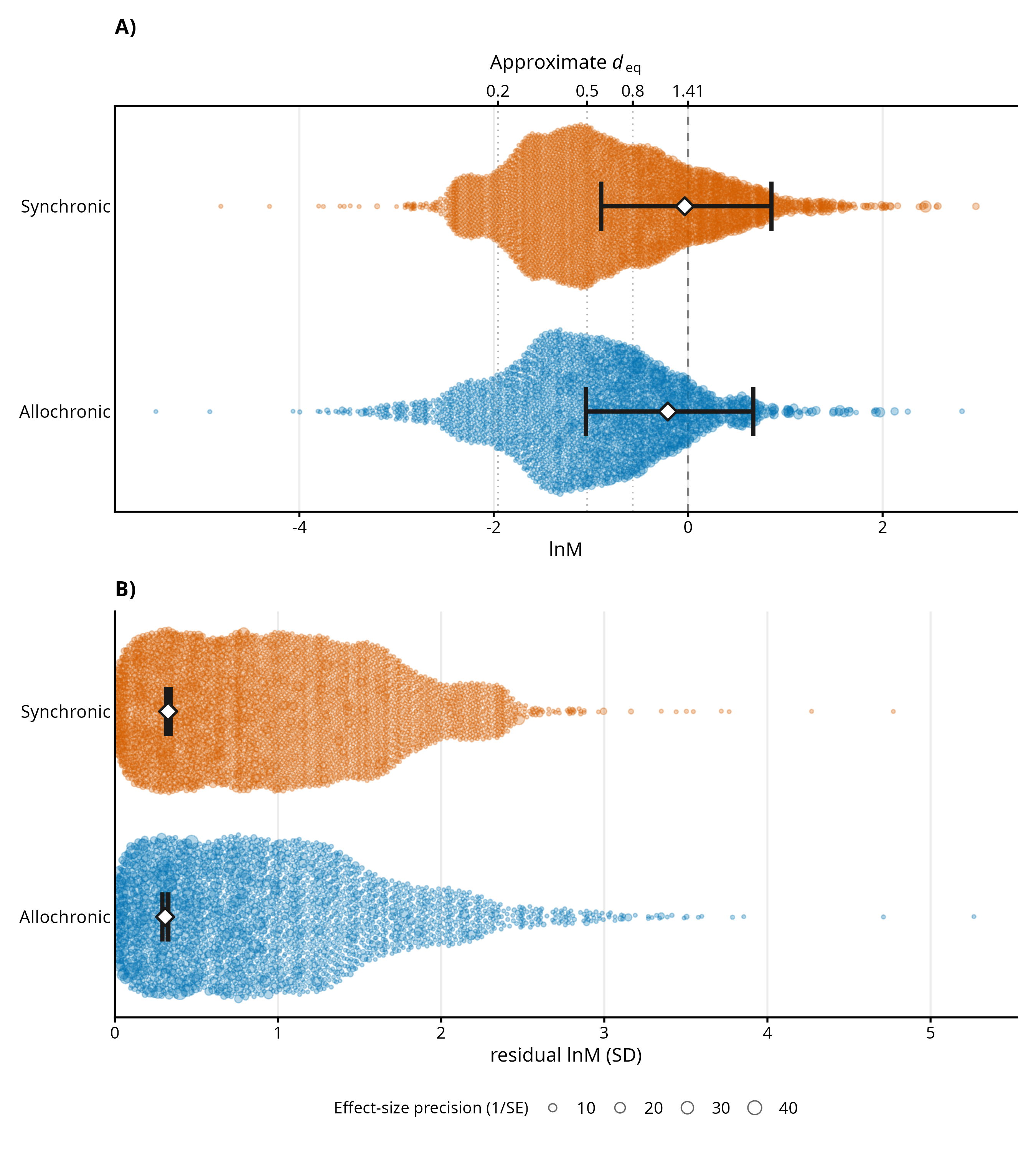
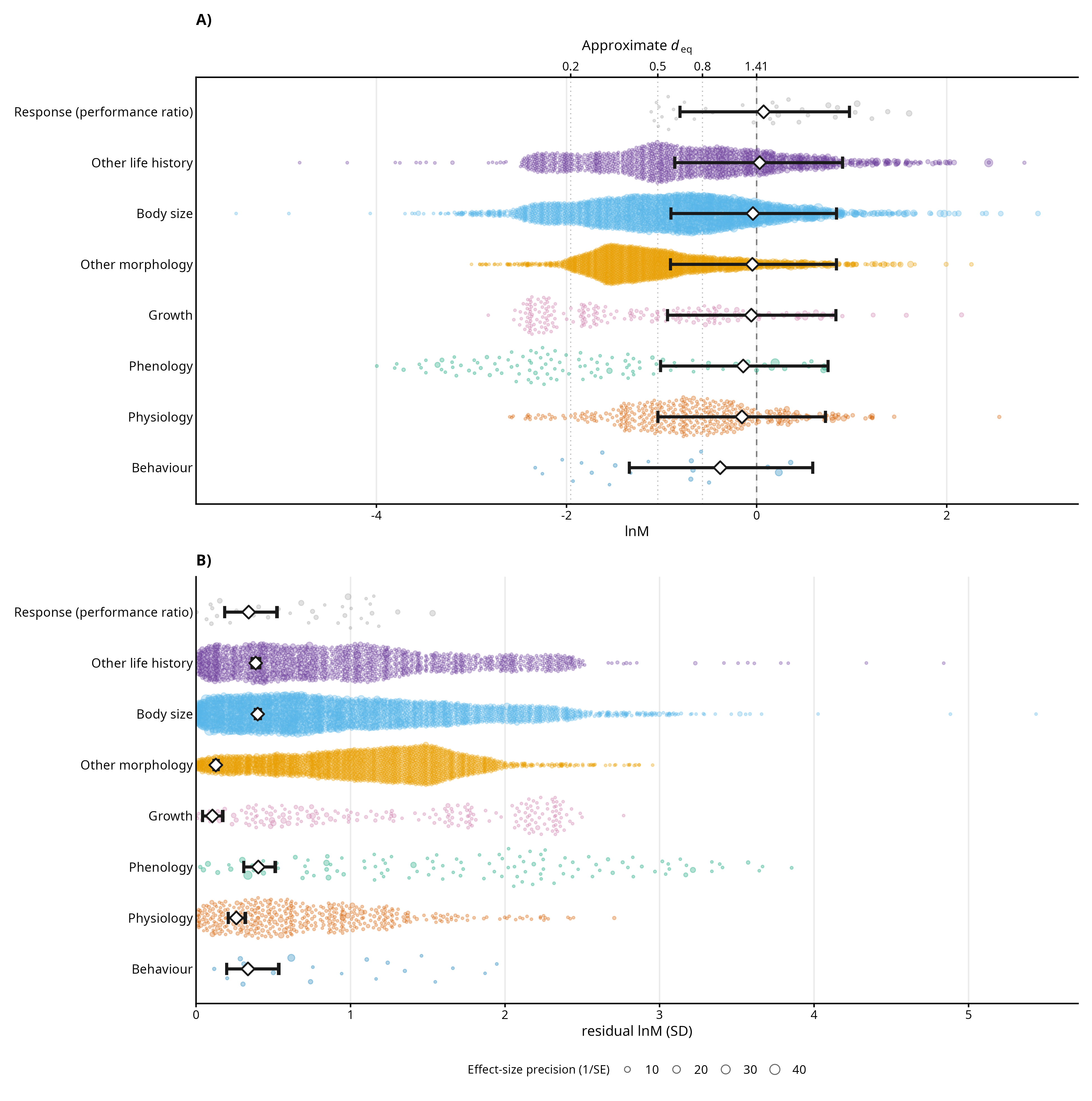
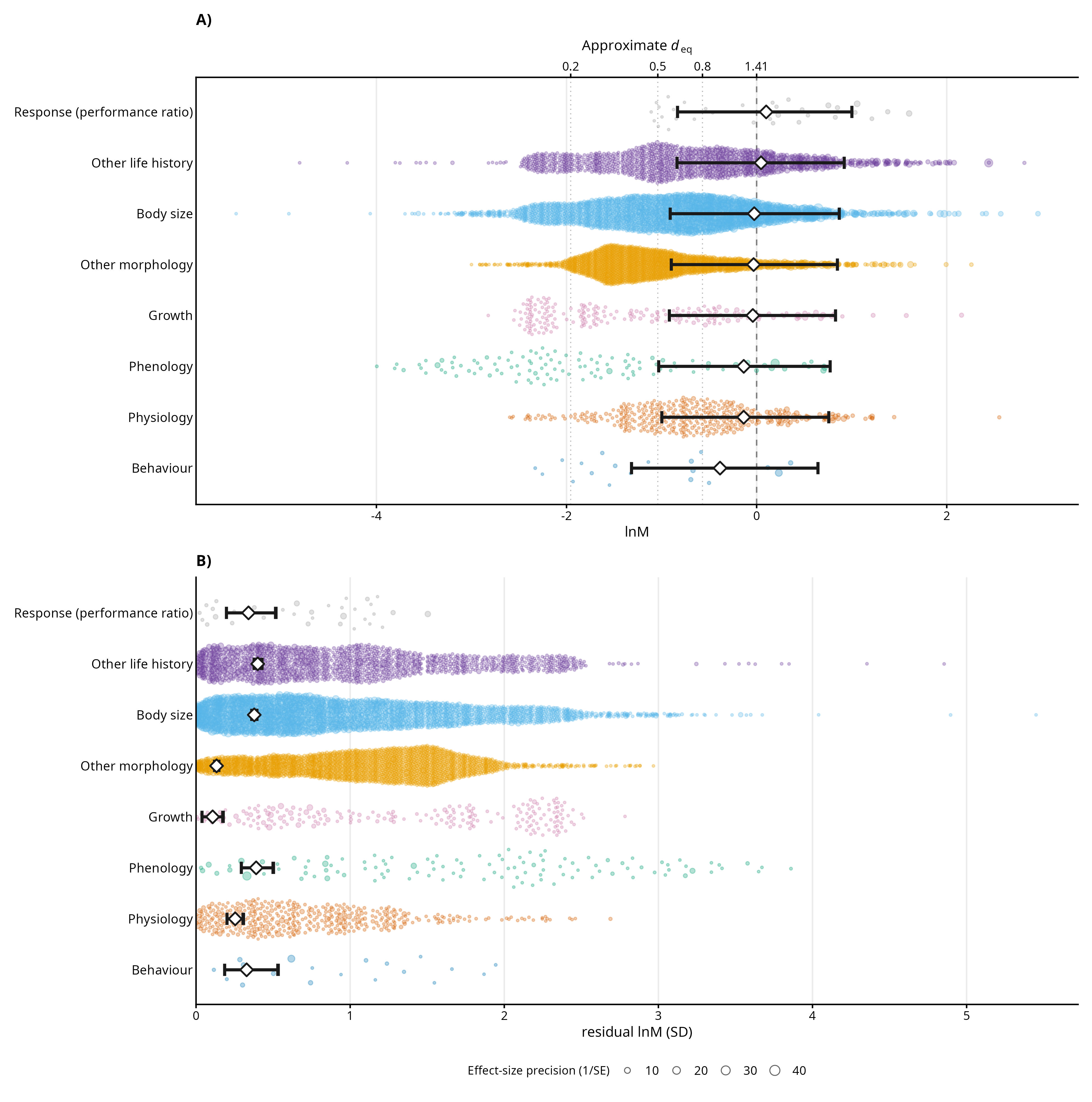
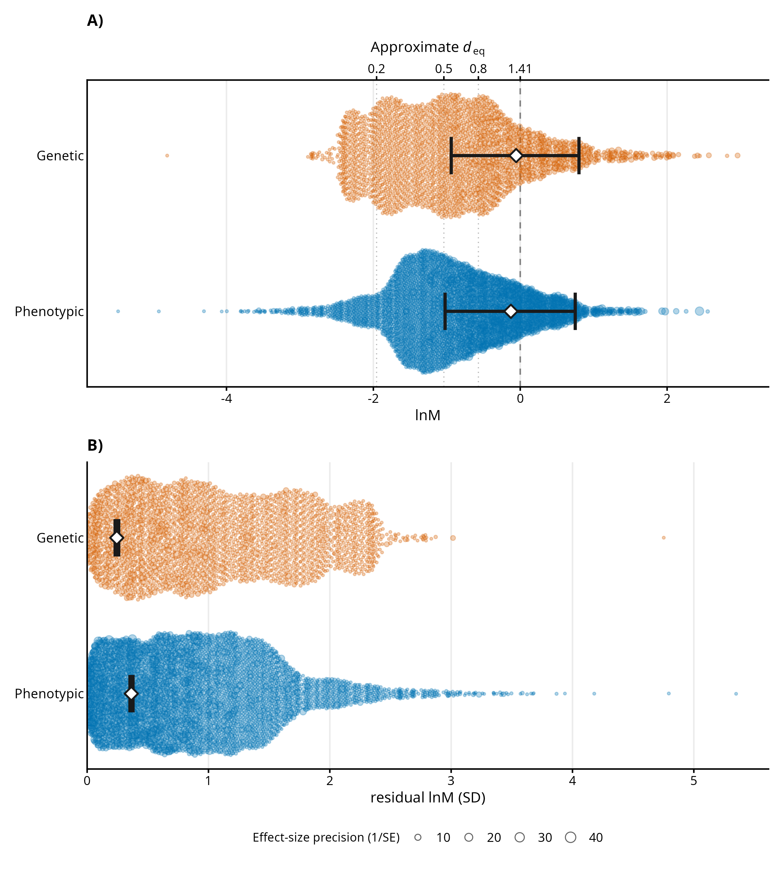
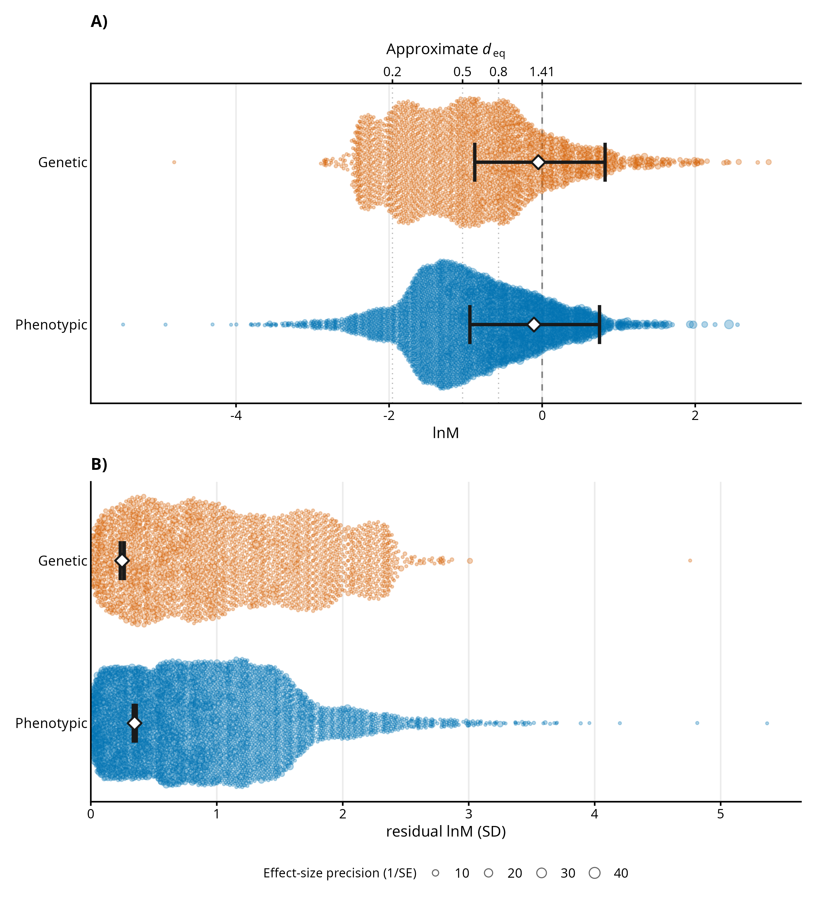
Each figure shows the focal moderator’s location (top) and scale (bottom) estimates from its additive model, with elapsed time held at its dataset mean. Points and beeswarm markers are on the same scale as the primary single-moderator orchard figures (see the model chapters); only the added time term differs.

Code
knitr::include_graphics(here::here("Rdata", "figures", "publication",
                                   "orchard_additive",
                                   "disturbance_plus_log10_years_orchard_combined.png"))

Code
knitr::include_graphics(here::here("Rdata", "figures", "publication",
                                   "orchard_additive",
                                   "disturbance_plus_log10_generations_orchard_combined.png"))

Code
knitr::include_graphics(here::here("Rdata", "figures", "publication",
                                   "orchard_additive",
                                   "design_plus_log10_years_orchard_combined.png"))

Code
knitr::include_graphics(here::here("Rdata", "figures", "publication",
                                   "orchard_additive",
                                   "design_plus_log10_generations_orchard_combined.png"))

Code
knitr::include_graphics(here::here("Rdata", "figures", "publication",
                                   "orchard_additive",
                                   "trait_type_plus_log10_years_orchard_combined.png"))

Code
knitr::include_graphics(here::here("Rdata", "figures", "publication",
                                   "orchard_additive",
                                   "trait_type_plus_log10_generations_orchard_combined.png"))

Code
knitr::include_graphics(here::here("Rdata", "figures", "publication",
                                   "orchard_additive",
                                   "genphen_plus_log10_years_orchard_combined.png"))

Code
knitr::include_graphics(here::here("Rdata", "figures", "publication",
                                   "orchard_additive",
                                   "genphen_plus_log10_generations_orchard_combined.png"))

WarningRead the diagnostics table before the figures above

The disturbance and trait_type models did not meet the convergence criteria used elsewhere in this book (max Rhat ≤ 1.01, bulk and tail ESS ≥ 400, and no divergent transitions) with either elapsed-time variable; the failures were most severe with log10_generations. Their summaries and figures are shown here for transparency, but should not be read as reliable estimates. The design and genphen models converged cleanly.