---
title: "Associations among moderators"
---
::: {.workflow}
::: {}
**Input**
Saved SAFE lnM dataset.
:::
::: {}
**Action**
Calculate pairwise association statistics.
:::
::: {}
**Output**
Three CSV tables and three plots.
:::
::: {}
**Next**
Build the dependency data.
:::
:::
```{r setup}
source(here::here("Scripts", "00_packages.R"))

continuous_vars <- c(
  log10_years = "Elapsed years",
  log10_generations = "Elapsed generations"
)

categorical_vars <- c(
  disturbance = "Disturbance context",
  design = "Comparison design",
  trait_type = "Trait type",
  genphen = "Study response",
  data_scale = "Measurement scale"
)

theme_association <- function(base_size = 15) {
  ggplot2::theme_minimal(base_size = base_size) +
    ggplot2::theme(
      plot.title = ggplot2::element_text(face = "bold", size = base_size + 3),
      plot.subtitle = ggplot2::element_text(colour = "grey30"),
      panel.grid.minor = ggplot2::element_blank(),
      legend.position = "bottom",
      axis.text = ggplot2::element_text(colour = "grey15"),
      strip.text = ggplot2::element_text(face = "bold")
    )
}

cramers_v_corrected <- function(x, y) {
  tab <- table(x, y)
  n <- sum(tab)
  if (n < 2L || nrow(tab) < 2L || ncol(tab) < 2L) return(NA_real_)
  chi <- suppressWarnings(stats::chisq.test(tab, correct = FALSE))
  phi2 <- unname(chi$statistic) / n
  r <- nrow(tab)
  k <- ncol(tab)
  phi2_corrected <- max(0, phi2 - ((k - 1) * (r - 1)) / (n - 1))
  r_corrected <- r - ((r - 1)^2) / (n - 1)
  k_corrected <- k - ((k - 1)^2) / (n - 1)
  denom <- min(k_corrected - 1, r_corrected - 1)
  if (denom <= 0) NA_real_ else sqrt(phi2_corrected / denom)
}

eta_squared_test <- function(y, group) {
  keep <- stats::complete.cases(y, group)
  y <- y[keep]
  group <- droplevels(factor(group[keep]))
  if (length(y) < 3L || nlevels(group) < 2L) {
    return(tibble::tibble(estimate = NA_real_, statistic = NA_real_, p_value = NA_real_))
  }
  fit <- stats::lm(y ~ group)
  tab <- stats::anova(fit)
  tibble::tibble(
    estimate = tab$`Sum Sq`[1] / sum(tab$`Sum Sq`),
    statistic = tab$`F value`[1],
    p_value = tab$`Pr(>F)`[1]
  )
}

significance_mark <- function(p) {
  dplyr::case_when(
    is.na(p) ~ "",
    p < 0.001 ~ "***",
    p < 0.01 ~ "**",
    p < 0.05 ~ "*",
    TRUE ~ ""
  )
}
```
## Action: association calculations
Association is measured on the scale appropriate to each pair: Pearson's *r* for two continuous variables, bias-corrected Cramér's *V* for two categorical variables, and the correlation ratio η² for a continuous variable grouped by a categorical variable.
The calculations treat contrasts as rows. They do not include the study,
system, or phylogenetic structures used later in the models. The reported
adjusted *p*-values use the Holm method within this chapter.
```{r load-data}
dat_es <- readRDS(here::here("Rdata", "effect_sizes", "proceed_lnm_safe.rds"))

figure_dir <- here::here("Rdata", "figures", "moderator_associations")
table_dir <- here::here("Rdata", "tables", "moderator_associations")
dir.create(figure_dir, recursive = TRUE, showWarnings = FALSE)
dir.create(table_dir, recursive = TRUE, showWarnings = FALSE)
```
## Continuous–continuous association
```{r continuous-analysis}
continuous_dat <- dat_es |>
  dplyr::select(dplyr::all_of(names(continuous_vars))) |>
  tidyr::drop_na()

pearson_test <- stats::cor.test(
  continuous_dat$log10_years,
  continuous_dat$log10_generations,
  method = "pearson"
)
spearman_test <- suppressWarnings(stats::cor.test(
  continuous_dat$log10_years,
  continuous_dat$log10_generations,
  method = "spearman",
  exact = FALSE
))

continuous_results <- tibble::tibble(
  method = c("Pearson", "Spearman sensitivity check"),
  estimate = c(unname(pearson_test$estimate), unname(spearman_test$estimate)),
  conf_low = c(pearson_test$conf.int[1], NA_real_),
  conf_high = c(pearson_test$conf.int[2], NA_real_),
  p_value = c(pearson_test$p.value, spearman_test$p.value),
  n = nrow(continuous_dat)
) |>
  dplyr::mutate(p_holm = stats::p.adjust(p_value, method = "holm"))

readr::write_csv(continuous_results, file.path(table_dir, "continuous_continuous.csv"))
knitr::kable(continuous_results, digits = 3,
             caption = "Continuous-moderator association and rank-based sensitivity check.")
```
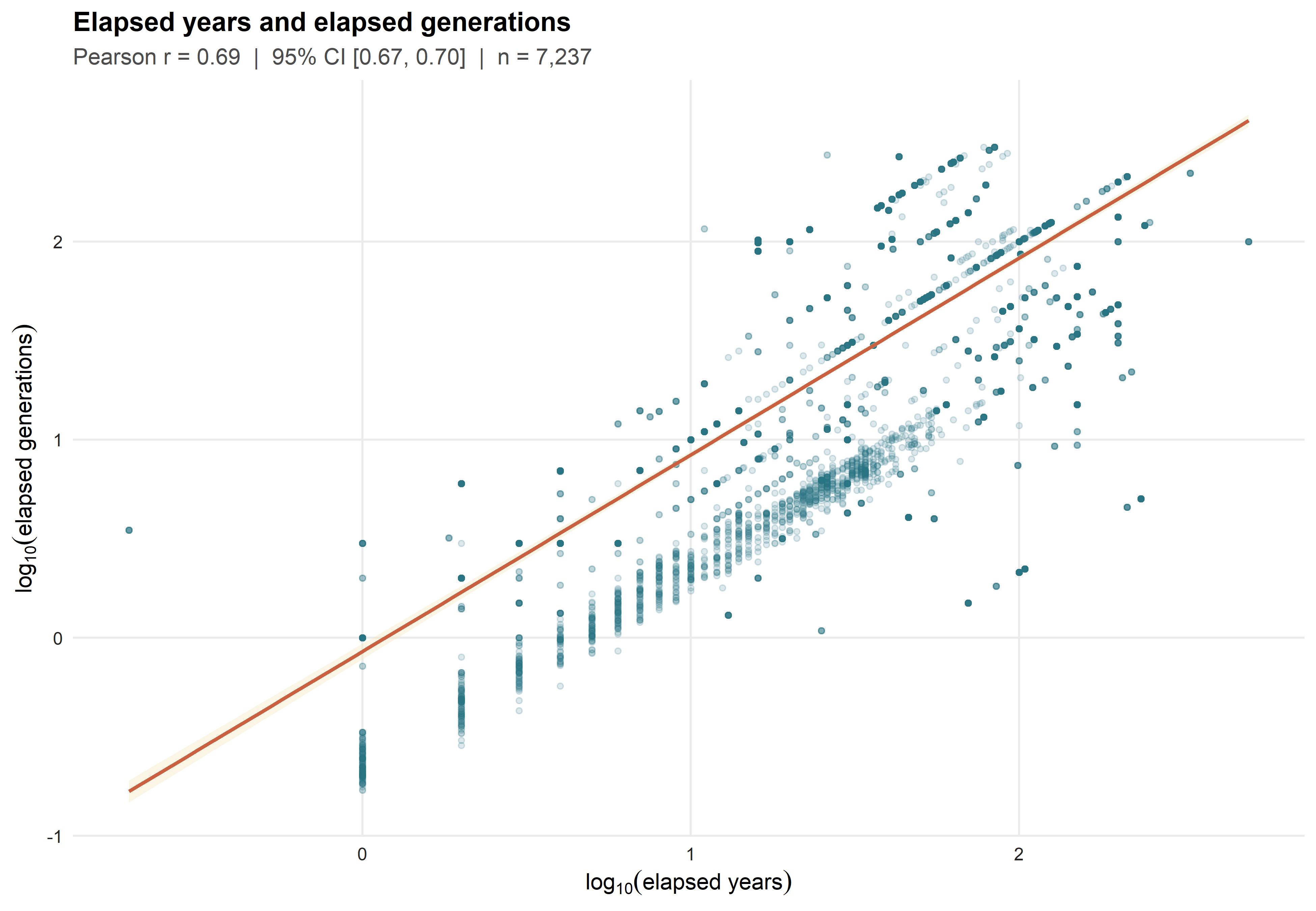
```{r continuous-plot, fig.width=13, fig.height=9, fig.cap="Association between elapsed time expressed in years and generations. The annotation reports Pearson's correlation and its 95% confidence interval."}
continuous_label <- sprintf(
  "Pearson r = %.2f  |  95%% CI [%.2f, %.2f]  |  n = %s",
  continuous_results$estimate[1], continuous_results$conf_low[1],
  continuous_results$conf_high[1], scales::comma(continuous_results$n[1])
)

p_continuous <- ggplot2::ggplot(
  continuous_dat,
  ggplot2::aes(x = log10_years, y = log10_generations)
) +
  ggplot2::geom_point(colour = "#257180", alpha = 0.16, size = 1.7) +
  ggplot2::geom_smooth(method = "lm", formula = y ~ x, se = TRUE,
                       colour = "#CB6040", fill = "#F2E5BF", linewidth = 1.3) +
  ggplot2::labs(
    title = "Elapsed years and elapsed generations",
    subtitle = continuous_label,
    x = expression(log[10]("elapsed years")),
    y = expression(log[10]("elapsed generations"))
  ) +
  theme_association(16)

ggplot2::ggsave(file.path(figure_dir, "continuous_continuous.png"), p_continuous,
                width = 13, height = 9, dpi = 320, bg = "white")
p_continuous
```
## Categorical–categorical associations
```{r categorical-analysis}
categorical_pairs <- utils::combn(names(categorical_vars), 2, simplify = FALSE)

categorical_results <- purrr::map_dfr(categorical_pairs, function(pair) {
  pair_dat <- dat_es |>
    dplyr::select(dplyr::all_of(pair)) |>
    tidyr::drop_na()
  tab <- table(pair_dat[[pair[1]]], pair_dat[[pair[2]]])
  chi <- suppressWarnings(stats::chisq.test(tab, correct = FALSE))
  tibble::tibble(
    variable_1 = pair[1], variable_2 = pair[2],
    label_1 = unname(categorical_vars[pair[1]]),
    label_2 = unname(categorical_vars[pair[2]]),
    cramers_v = cramers_v_corrected(pair_dat[[pair[1]]], pair_dat[[pair[2]]]),
    chi_square = unname(chi$statistic), df = unname(chi$parameter),
    p_value = chi$p.value, n = nrow(pair_dat),
    min_expected = min(chi$expected)
  )
}) |>
  dplyr::mutate(
    p_holm = stats::p.adjust(p_value, method = "holm"),
    stars = significance_mark(p_holm),
    tile_label = sprintf("%.2f%s", cramers_v, stars)
  )

readr::write_csv(categorical_results, file.path(table_dir, "categorical_categorical.csv"))
knitr::kable(
  categorical_results |>
    dplyr::select(label_1, label_2, cramers_v, chi_square, df, p_value, p_holm, n, min_expected),
  digits = 3,
  caption = "Pairwise categorical associations. Cramér's V is bias-corrected; p-values are from Pearson chi-square tests."
)
```
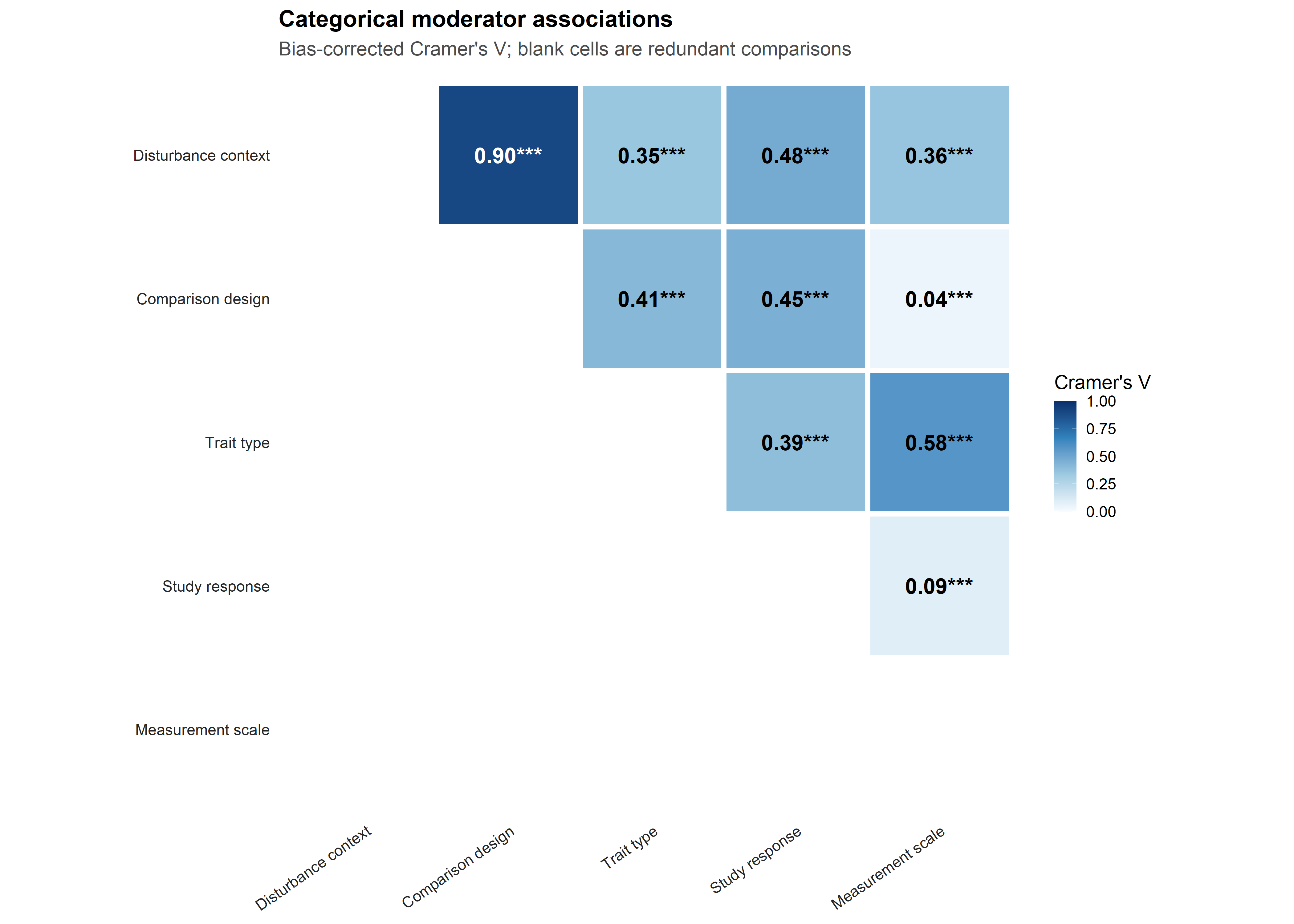
`r sum(categorical_results$min_expected < 5)` of `r nrow(categorical_results)` categorical comparisons contain at least one expected cell count below five. Their chi-square *p*-values are based on these small expected counts.
```{r categorical-plot, fig.width=14, fig.height=10, fig.cap="Bias-corrected Cramér's V among categorical moderators. Stars denote Holm-adjusted significance: * p < .05, ** p < .01, *** p < .001."}
cat_levels <- unname(categorical_vars)
p_categorical <- ggplot2::ggplot(
  categorical_results,
  ggplot2::aes(
    x = factor(label_2, levels = cat_levels),
    y = factor(label_1, levels = rev(cat_levels)),
    fill = cramers_v
  )
) +
  ggplot2::geom_tile(colour = "white", linewidth = 2) +
  ggplot2::geom_text(ggplot2::aes(label = tile_label, colour = cramers_v > 0.65),
                     fontface = "bold", size = 6) +
  ggplot2::scale_fill_gradientn(
    colours = c("#F7FBFF", "#9ECAE1", "#3182BD", "#08306B"),
    limits = c(0, 1), name = "Cramer's V"
  ) +
  ggplot2::scale_colour_manual(values = c(`FALSE` = "black", `TRUE` = "white"), guide = "none") +
  ggplot2::scale_x_discrete(drop = FALSE) +
  ggplot2::scale_y_discrete(drop = FALSE) +
  ggplot2::coord_fixed() +
  ggplot2::labs(
    title = "Categorical moderator associations",
    subtitle = "Bias-corrected Cramer's V; blank cells are redundant comparisons",
    x = NULL, y = NULL
  ) +
  theme_association(15) +
  ggplot2::theme(
    axis.text.x = ggplot2::element_text(angle = 35, hjust = 1),
    panel.grid = ggplot2::element_blank(),
    legend.position = "right"
  )

ggplot2::ggsave(file.path(figure_dir, "categorical_categorical.png"), p_categorical,
                width = 14, height = 10, dpi = 320, bg = "white")
p_categorical
```
## Continuous–categorical associations
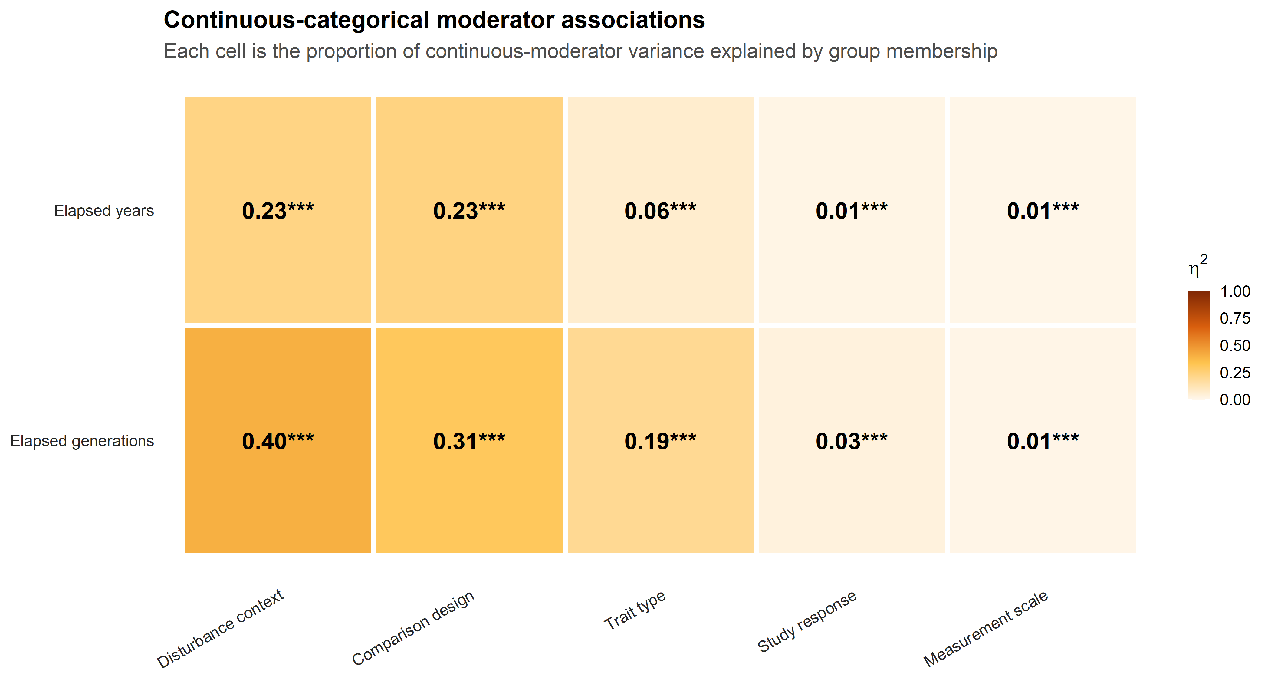
For each mixed pair, η² is the proportion of variation in the continuous moderator explained by the categorical grouping in a one-way model. Because η² is non-negative, the heatmap shows strength but not direction.
```{r mixed-analysis}
mixed_grid <- tidyr::crossing(
  continuous = names(continuous_vars),
  categorical = names(categorical_vars)
)

mixed_results <- purrr::pmap_dfr(mixed_grid, function(continuous, categorical) {
  result <- eta_squared_test(dat_es[[continuous]], dat_es[[categorical]])
  result |>
    dplyr::mutate(
      continuous = continuous,
      categorical = categorical,
      continuous_label = unname(continuous_vars[continuous]),
      categorical_label = unname(categorical_vars[categorical]),
      n = sum(stats::complete.cases(dat_es[[continuous]], dat_es[[categorical]])),
      groups = nlevels(droplevels(factor(dat_es[[categorical]])))
    )
}) |>
  dplyr::mutate(
    p_holm = stats::p.adjust(p_value, method = "holm"),
    stars = significance_mark(p_holm),
    tile_label = sprintf("%.2f%s", estimate, stars)
  )

readr::write_csv(mixed_results, file.path(table_dir, "continuous_categorical.csv"))
knitr::kable(
  mixed_results |>
    dplyr::select(continuous_label, categorical_label, estimate, statistic,
                  p_value, p_holm, n, groups),
  digits = 3,
  col.names = c("Continuous moderator", "Categorical moderator", "Eta squared",
                "F", "p", "Holm p", "n", "Groups"),
  caption = "Mixed-variable associations. Eta squared is based on a one-way linear model."
)
```
```{r mixed-plot, fig.width=14, fig.height=7.5, fig.cap="Correlation ratio η² for every continuous–categorical moderator pair. Stars denote Holm-adjusted significance: * p < .05, ** p < .01, *** p < .001."}
p_mixed <- ggplot2::ggplot(
  mixed_results,
  ggplot2::aes(
    x = factor(categorical_label, levels = unname(categorical_vars)),
    y = factor(continuous_label, levels = rev(unname(continuous_vars))),
    fill = estimate
  )
) +
  ggplot2::geom_tile(colour = "white", linewidth = 2) +
  ggplot2::geom_text(ggplot2::aes(label = tile_label), fontface = "bold", size = 6.5) +
  ggplot2::scale_fill_gradientn(
    colours = c("#FFF7EC", "#FEC44F", "#D95F0E", "#7F2704"),
    limits = c(0, 1), name = expression(eta^2)
  ) +
  ggplot2::labs(
    title = "Continuous-categorical moderator associations",
    subtitle = "Each cell is the proportion of continuous-moderator variance explained by group membership",
    x = NULL, y = NULL
  ) +
  theme_association(16) +
  ggplot2::theme(
    axis.text.x = ggplot2::element_text(angle = 30, hjust = 1),
    panel.grid = ggplot2::element_blank(),
    legend.position = "right"
  )

ggplot2::ggsave(file.path(figure_dir, "continuous_categorical.png"), p_mixed,
                width = 14, height = 7.5, dpi = 320, bg = "white")
p_mixed
```