---
title: "Small-study effects diagnostic"
---
::: {.workflow}
::: {}
**Input**
SAFE lnM estimates, group sample sizes, and the phylogenetic covariance matrix.
:::
::: {}
**Action**
Fit sample-size-based Egger-style location–scale meta-regressions.
:::
::: {}
**Output**
Small-study slope, infinite-sample intercept, and diagnostic plot.
:::
::: {}
**Next**
Check whether conclusions are robust to alternative analysis specifications.
:::
:::
```{r setup, include=FALSE}
source(here::here("Scripts", "00_packages.R"))
source(here::here("Scripts", "20_small_study_effects.R"))
cache_se <- read_small_study_cache("n_se_sigmax")
cache_v <- read_small_study_cache("n_v_sigma1")
missing_caches <- c("n_se_sigmax", "n_v_sigma1")[c(is.null(cache_se), is.null(cache_v))]
if (length(missing_caches) > 0) {
stop(
"Small-study brms caches are missing: ",
paste(missing_caches, collapse = ", "),
". Fit on the remote server with remote_run_small_study_brms_parallel.sh, build the ",
"caches with remote_precompute_small_study_brms_cache.R, then copy them ",
"into Rdata/epred_draws/.",
call. = FALSE
)
}
figure_path <- here::here("Rdata", "figures", "publication", "small_study_effects.png")
crosscheck_path <- here::here("Rdata", "tables", "small_study_effects.csv")
crosscheck <- if (file.exists(crosscheck_path)) {
readr::read_csv(crosscheck_path, show_col_types = FALSE)
} else {
NULL
}
```
## Predictor: sample size rather than sampling error
We assess whether estimated effect magnitudes vary systematically with study
size. Such a pattern is a **small-study effect**. It is a diagnostic, not a direct test of the
publication process.
The usual Egger regression uses an effect's sampling standard error as the
predictor. For lnM, however, the effect and its estimated standard error share
underlying variance components. Following the
[lnM worked example](https://itchyshin.github.io/meta-analysis_of_magnitude/)
and Nakagawa et al. (2022), we instead use a predictor calculated only from the
two group sample sizes.
For each contrast, the harmonic-mean sample size is
$$
n_0 = \frac{2 n_1 n_2}{n_1 + n_2},
$$
and the predictors are built from the **half** harmonic-mean sample size
$$
\tilde{n}_0 = \frac{n_0}{2} = \frac{n_1 n_2}{n_1 + n_2}.
$$
We fit two related models:
1. $1/\sqrt{\tilde{n}_0}$ is an SE analogue; its slope is the primary
diagnostic for small-study effects.
2. $1/\tilde{n}_0$ is a variance analogue; its intercept at $1/\tilde{n}_0=0$
is an infinite-sample, bias-adjusted estimate. We treat this as a
conditional sensitivity estimate rather than an automatic replacement for
the primary meta-analytic mean.
### Constructing the predictors
The two predictors are calculated directly from the original group sample
sizes. Neither uses the observed lnM estimate or its sampling variance.
```{r predictor-code, eval=FALSE}
diagnostic_data <- readRDS(
  here::here("Rdata", "effect_sizes", "proceed_lnm_safe.rds")
) |>
  dplyr::filter(
    is.finite(n1), n1 > 0,
    is.finite(n2), n2 > 0
  ) |>
  dplyr::mutate(
    # Half harmonic-mean sample size, n0_tilde = n0 / 2.
    n0_tilde = (n1 * n2) / (n1 + n2),
    n_se     = 1 / sqrt(n0_tilde),
    n_v      = 1 / n0_tilde
  )
```
## Model structure
Both models use SAFE lnM as the response and retain the analysis's known
sampling variances through the effect-size covariance matrix `V`. Random
intercepts account for clustering by reference, phylogenetically correlated
species, and effect-size record. Thus the diagnostic changes the fixed
predictor while preserving the main sources of non-independence.
```{r model-code, eval=FALSE}
formula_se <- brms::bf(
  yi_lnM_safe ~ n_se + (1 | ref_id) +
    (1 | gr(sp_ncbi, cov = A)) + (1 | gr(es_id_model, cov = V)),
  sigma ~ n_se
)

fit_se <- brms::brm(
  formula_se, data = dat_model, data2 = list(A = A_mod, V = V)
)

formula_v <- brms::bf(
  yi_lnM_safe ~ n_v + (1 | ref_id) +
    (1 | gr(sp_ncbi, cov = A)) + (1 | gr(es_id_model, cov = V)),
  sigma ~ 1
)

fit_v <- brms::brm(
  formula_v, data = dat_model, data2 = list(A = A_mod, V = V)
)
```
### Specification grid
Each predictor was crossed with two scale specifications — a constant residual
SD (`sigma ~ 1`) and one varying with the predictor (`sigma ~ x`) — giving four
fits. `remote_fit_one_small_study_brms.R` writes a model only after it passes
fixed convergence criteria: no divergent transitions, $\hat{R} \le 1.01$, and
bulk and tail ESS of at least 400.
| Model | Predictor | Scale | Status |
|---|---|---|---|
| `n_se_sigmax` | $1/\sqrt{\tilde{n}_0}$ | `sigma ~ n_se` | Reported below |
| `n_v_sigma1` | $1/\tilde{n}_0$ | `sigma ~ 1` | Reported below |
| `n_se_sigma1` | $1/\sqrt{\tilde{n}_0}$ | `sigma ~ 1` | Criteria not met; refit pending |
| `n_v_sigmax` | $1/\tilde{n}_0$ | `sigma ~ n_v` | Criteria not met; refit pending |
The two reported models are fitted to
**`r format(cache_se$meta$n_obs, big.mark = ",")` contrasts** with complete,
positive group sample sizes and resolved species names.
## Results
### Convergence
```{r convergence-table}
diag_tbl <- dplyr::bind_rows(cache_se$diagnostics, cache_v$diagnostics) |>
  dplyr::select(
    Model = model_id, Moderator = moderator,
    `Max Rhat` = max_rhat, `Min bulk ESS` = min_bulk_ess,
    `Min tail ESS` = min_tail_ess, Divergences = n_divergent,
    `Treedepth hits` = max_treedepth_hits
  ) |>
  dplyr::mutate(
    `Max Rhat` = round(`Max Rhat`, 4),
    dplyr::across(dplyr::starts_with("Min"), ~ round(.x, 0))
  )

knitr::kable(
  diag_tbl,
  caption = "Sampler diagnostics for the two reported models."
)
```
### Model summaries
Complete `summary()` output is read from the cached draw objects; the ~400 MB
`brms` fits are not loaded at render.
```{r model-summary-se}
writeLines(cache_se$summary_txt)
```
```{r model-summary-v}
writeLines(cache_v$summary_txt)
```
### Coefficient table
```{r results-table}
knitr::kable(
  small_study_coef_table(list(cache_se, cache_v)),
  digits = 3,
  caption = paste0(
    "Posterior fixed effects with 95% equal-tailed credible intervals. The ",
    "primary diagnostic is the $1/\\sqrt{\\tilde{n}_0}$ location slope; the ",
    "$1/\\tilde{n}_0$ intercept estimates the effect at infinite sample size."
  )
)
```
## Diagnostic plot
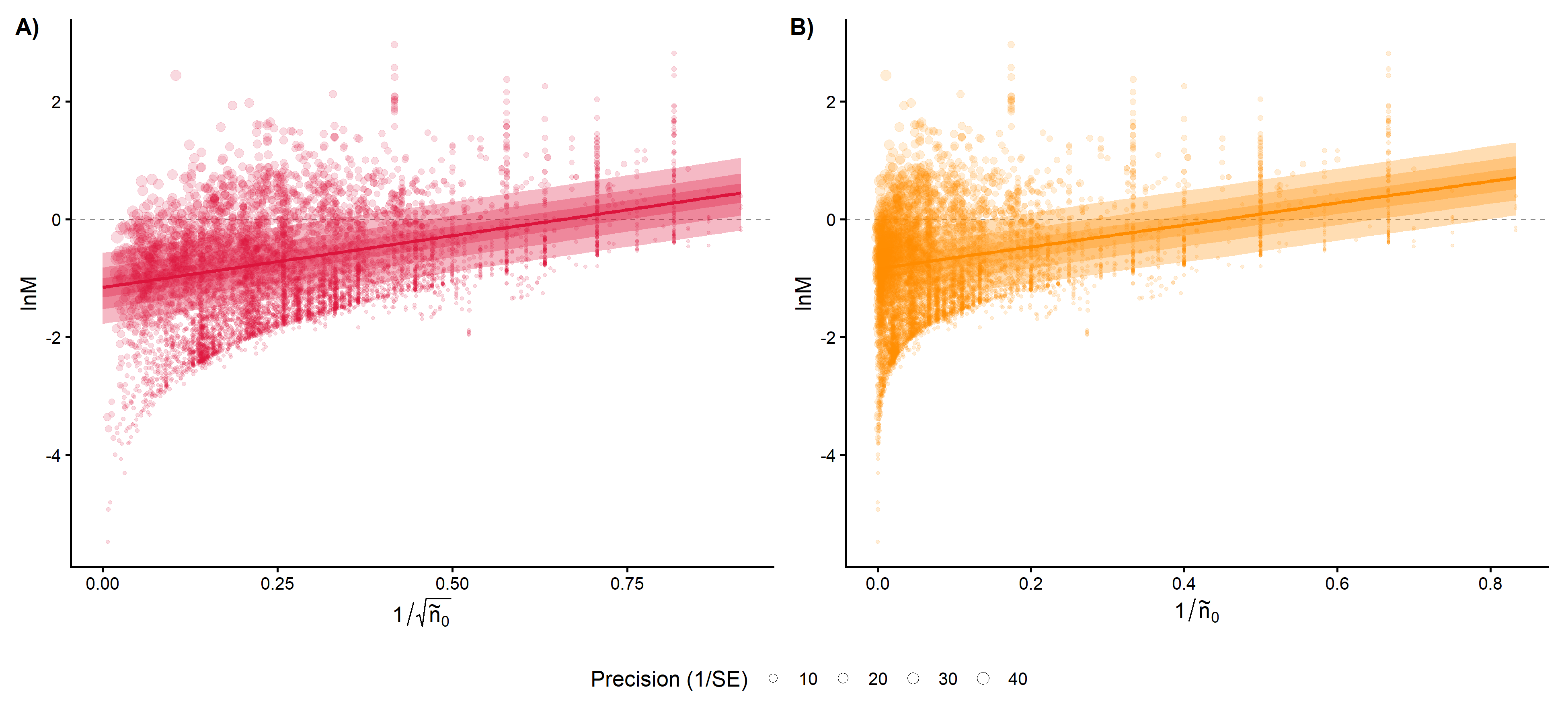
The two panels are constructed from the cached draws and joined with
`patchwork`. Bubble area represents sampling precision, $1/\mathrm{SE}$. Bands
show 50%, 80%, and 95% credible intervals for the posterior mean, drawn down to
the predictor's zero bound.
```{r figure-code, eval=FALSE}
p_se <- build_small_study_location_panel(cache_se, show_legend = TRUE)
p_v <- build_small_study_location_panel(cache_v, show_legend = FALSE)

p <- ((p_se + p_v) / patchwork::guide_area()) +
  patchwork::plot_layout(heights = c(1, 0.10), guides = "collect") +
  patchwork::plot_annotation(tag_levels = "A", tag_suffix = ")") &
  ggplot2::theme(
    legend.position = "bottom",
    legend.justification = "center",
    plot.tag = ggplot2::element_text(face = "bold", size = 14),
    plot.tag.position = c(0.01, 0.99)
  )

ggplot2::ggsave(
  here::here("Rdata", "figures", "publication", "small_study_effects.png"),
  p, width = 13, height = 6, dpi = 300, bg = "white"
)
```
```{r figure, fig.width=13, fig.height=6}
p <- build_small_study_brms_figure(cache_se, cache_v)

dir.create(dirname(figure_path), recursive = TRUE, showWarnings = FALSE)
ggplot2::ggsave(figure_path, p, width = 13, height = 6, dpi = 300, bg = "white")

p
```
::: {.callout-note}
The infinite-sample intercept is an extrapolation to $1/\tilde{n}_0=0$, outside
the observed finite-sample data. It is reported as a sensitivity analysis.
:::
### Residual SD across study size
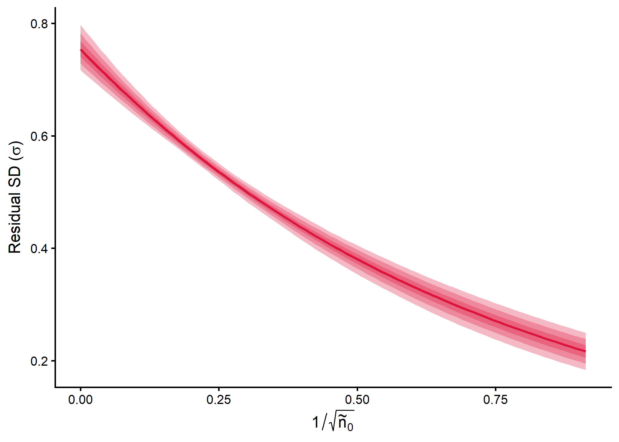
`n_se_sigmax` models the residual SD as a function of the predictor. The
posterior for that scale submodel is plotted below.
```{r scale-figure, fig.width=7, fig.height=5}
build_small_study_scale_panel(cache_se)
```
## Frequentist cross-check
`metafor::rma.mv` fits the same location structure by REML and is
homoscedastic, so it corresponds to the `sigma ~ 1` specification.
```{r crosscheck-table}
if (is.null(crosscheck)) {
  cat("Cross-check table not available.\n")
} else {
  knitr::kable(
    crosscheck |>
      dplyr::mutate(
        # The predictor is carried by the Term column, so the model label only
        # needs its role. Both the current and regenerated CSV spellings map
        # here, since the cached table predates the notation fix.
        model = dplyr::recode(
          model,
          `Small-study slope: 1 / sqrt(n0)` = "Small-study slope",
          `Small-study slope: 1 / sqrt(n0_tilde)` = "Small-study slope",
          `Adjustment model: 1 / n0` = "Adjustment model",
          `Adjustment model: 1 / n0_tilde` = "Adjustment model"
        ),
        term = dplyr::recode(
          term,
          intrcpt = "Intercept",
          n_se = "$1/\\sqrt{\\tilde{n}_0}$ slope",
          n_v = "$1/\\tilde{n}_0$ slope"
        ),
        dplyr::across(c(estimate, std_error, ci_lower, ci_upper), ~ round(.x, 3))
      ) |>
      dplyr::select(
        Model = model, Term = term, Estimate = estimate,
        `Standard error` = std_error, `95% CI lower` = ci_lower,
        `95% CI upper` = ci_upper
      ),
    caption = "REML cross-check (metafor::rma.mv, homoscedastic)."
  )
}
```
## Reproduce the cached outputs
Normal book renders read the small draw caches under `Rdata/epred_draws/`. The
fits themselves are run on a remote server:
```bash
# 1. Fit the specification grid (four models, parallel)
bash remote_run_small_study_brms_parallel.sh

# 2. Build the small draw caches from the fits that converged
Rscript Scripts/remote_precompute_small_study_brms_cache.R

# 3. Copy the caches into the book mirror
scp remote-server:'~/Documents/PACE/outputs/epred_draws/small_study_*.rds' Rdata/epred_draws/
```
To regenerate the REML cross-check locally:
```{r reproduce, eval=FALSE}
source(here::here("Scripts", "00_packages.R"))
source(here::here("Scripts", "20_small_study_effects.R"))
run_small_study_analysis()
```