---
title: "Elapsed time (log₁₀ years)"
---
::: {.workflow}
::: {}
**Input**
Saved prediction and summary files.
:::
::: {}
**Action**
Read the model record and build its figure.
:::
::: {}
**Output**
Model table, checks, and plot.
:::
::: {}
**Next**
Continue to the next model chapter.
:::
:::
```{r setup, include=FALSE}
source(here::here("Scripts", "14_epred_cache.R"))
cache_dir <- here::here("Rdata", "epred_draws")
cache <- read_epred_cache("m03", cache_dir)
```
## Phylogenetic covariance and model species
This model contains **253 species** (7,186 contrasts). The phylogenetic correlation matrix was constructed and aligned to those species as follows; `brms` uses it in `(1 | gr(sp_ncbi, cov = A))`.
```{r phylogenetic-covariance, eval=FALSE}
A_full <- prepR4pcm::pr_phylo_cor(tree_final)
# Fallback if needed: ape::vcv.phylo(tree_final, corr = TRUE)
dat_model <- dat_es |> dplyr::filter(!is.na(log10_years))
phylo <- prepare_phylo_and_data(dat_model, A_full, fill_unmatched = TRUE)
dat_model <- phylo$dat_model
A <- phylo$A_mod
formula <- brms::bf(
  yi_lnM_safe ~ log10_years + (1 | ref_id) +
    (1 | gr(sp_ncbi, cov = A)) + (1 | gr(es_id_model, cov = V)),
  sigma ~ log10_years
)
V <- phylo$V
fit <- brms::brm(formula, data = dat_model,
                 data2 = list(A = A, V = V))
```
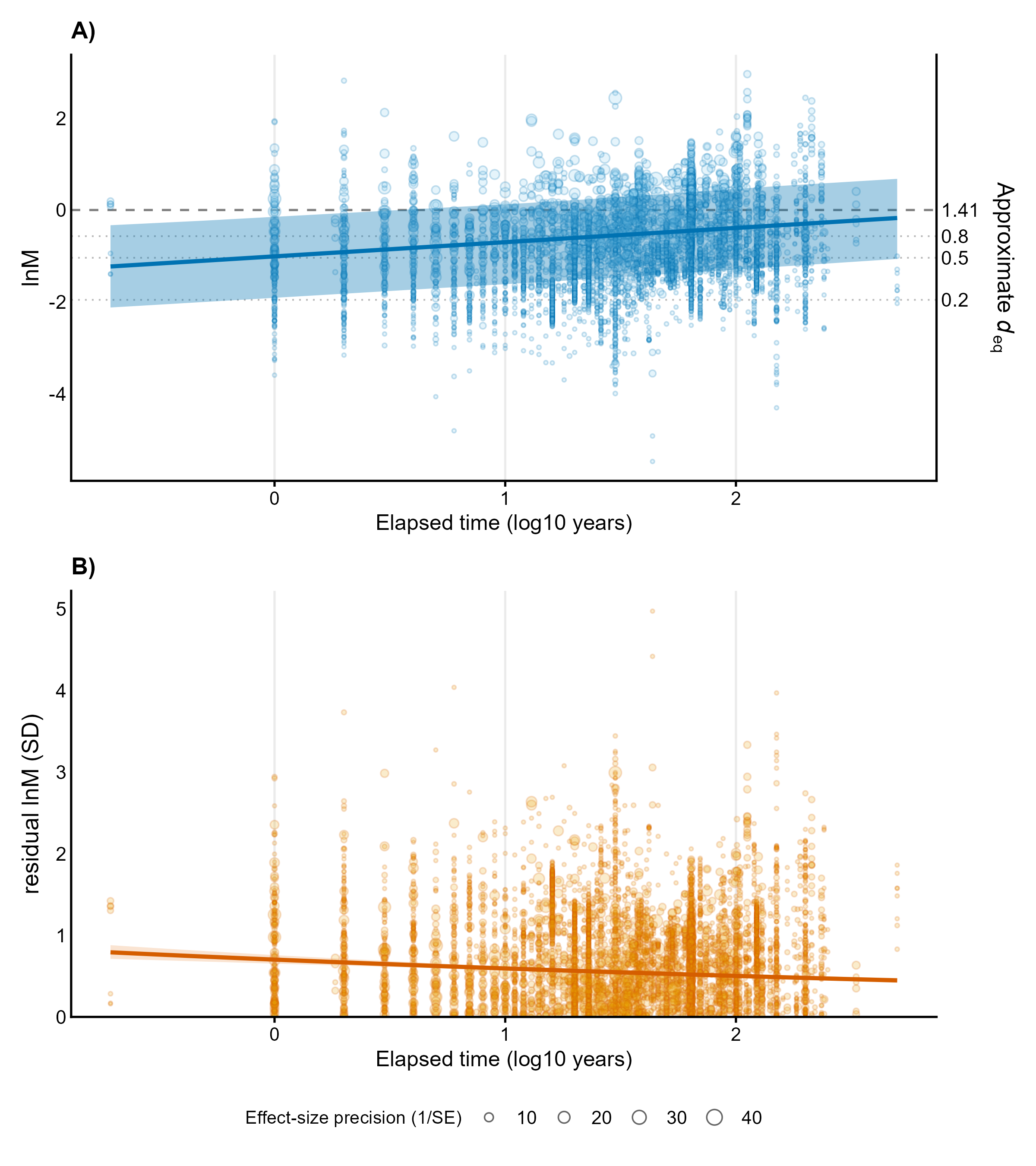
Continuous moderator: divergence as a function of elapsed time in years (log₁₀).
## Model summary
`summary()` is read from `Rdata/epred_draws/m03.rds`; the full `brms` fit is not loaded at render.
```{r summary}
print_cache_summary(cache)
```
## Main predictions in equivalent-d units
Predictions at 1, 10, and 100 years are reported on the $\ln M$ scale and as
$d_{\mathrm{eq}} \approx \sqrt{2\exp(2\ln M)}$. These are prediction-scale
summaries from the cached posterior draws; the regression slope itself is not
transformed into an equivalent $d$.
```{r elapsed-years-d-eq}
source(here::here("Scripts", "18_contrasts_cache.R"))
kable_contrasts(
  format_continuous_d_eq(cache, unit = "Years"),
  caption = "Predicted lnM and equivalent d at selected elapsed years, with 95% credible intervals."
)
```
## Orchard-like model figure
The orchard-style figure is read from `Rdata/figures/publication/orchard/`. The complete editable code used to build this plot is shown below.
```{r figure, fig.width=8, fig.height=9}
knitr::include_graphics(
  here::here("Rdata", "figures", "publication", "orchard", "m03_orchard_combined.png")
)
```
### Editable plotting code
```{r build-orchard-m03, eval=FALSE}
library(here)
library(tidyverse)
library(patchwork)

model_id <- "m03"
moderator <- "log10_years"
moderator_label <- "Elapsed time (log10 years)"
col_location <- "#0072B2"
col_location_light <- "#88CCEE"
col_scale <- "#D55E00"
col_scale_light <- "#E69F00"
col_scale_ribbon <- "#F2B27E"

out_dir <- here::here("Rdata", "figures", "publication", "orchard")
out_dir_pdf <- here::here("Figures", "publication", "orchard")
dir.create(out_dir, recursive = TRUE, showWarnings = FALSE)
dir.create(out_dir_pdf, recursive = TRUE, showWarnings = FALSE)

dat_es <- readRDS(here::here("Rdata", "effect_sizes", "proceed_lnm_safe.rds"))
cache <- readRDS(here::here("Rdata", "epred_draws", paste0(model_id, ".rds")))

theme_orchard <- function() {
  ggplot2::theme_classic(base_size = 13) +
    ggplot2::theme(
      axis.text.y        = ggplot2::element_text(size = 11),
      axis.title.x       = ggplot2::element_text(size = 12),
      axis.ticks.y       = ggplot2::element_blank(),
      panel.grid.major.x = ggplot2::element_line(colour = "grey92"),
      legend.position    = "bottom",
      legend.title       = ggplot2::element_text(size = 10),
      plot.title         = ggplot2::element_text(size = 13, face = "bold"),
      plot.caption       = ggplot2::element_text(size = 9, colour = "grey50")
    )
}

save_plot <- function(p, stem, width = 8, height = 6) {
  ggplot2::ggsave(file.path(out_dir_pdf, paste0(stem, ".pdf")), p,
                  width = width, height = height, device = cairo_pdf)
  ggplot2::ggsave(file.path(out_dir, paste0(stem, ".png")), p,
                  width = width, height = height, dpi = 300, type = "cairo")
}

raw <- dat_es[!is.na(dat_es[[moderator]]), ] |>
  dplyr::mutate(precision = 1 / sqrt(vi_lnM_safe))

pred <- cache$loc |>
  dplyr::group_by(.data[[moderator]]) |>
  dplyr::summarise(
    estimate = mean(.epred),
    lowerCL = quantile(.epred, 0.025),
    upperCL = quantile(.epred, 0.975),
    .groups = "drop"
  )

pred_sig <- cache$scl |>
  dplyr::group_by(.data[[moderator]]) |>
  dplyr::summarise(
    estimate = mean(sigma),
    lowerCL = quantile(sigma, 0.025),
    upperCL = quantile(sigma, 0.975),
    .groups = "drop"
  )

raw_pred_loc <- approx(
  pred[[moderator]], pred$estimate,
  xout = raw[[moderator]], rule = 2
)$y

raw_cont_sig <- raw |>
  dplyr::mutate(abs_resid = abs(yi_lnM_safe - raw_pred_loc))

p_loc <- ggplot2::ggplot() +
  ggplot2::geom_hline(yintercept = 0, linetype = "dashed", colour = "grey50") +
  ggplot2::geom_point(
    data = raw,
    ggplot2::aes(x = .data[[moderator]], y = yi_lnM_safe, size = precision),
    alpha = 0.22, shape = 21, fill = col_location_light, colour = col_location
  ) +
  ggplot2::geom_ribbon(
    data = pred,
    ggplot2::aes(x = .data[[moderator]], ymin = lowerCL, ymax = upperCL),
    alpha = 0.35, fill = col_location
  ) +
  ggplot2::geom_line(
    data = pred,
    ggplot2::aes(x = .data[[moderator]], y = estimate),
    linewidth = 1.1, colour = col_location
  ) +
  ggplot2::scale_size_continuous(name = "Precision (1/SE)", range = c(0.3, 4)) +
  ggplot2::labs(
    x = moderator_label,
    y = "lnM",
    title = NULL
  ) +
  theme_orchard()

p_scl <- ggplot2::ggplot() +
  ggplot2::geom_point(
    data = raw_cont_sig,
    ggplot2::aes(x = .data[[moderator]], y = abs_resid, size = precision),
    alpha = 0.20, shape = 21, fill = col_scale_light, colour = col_scale
  ) +
  ggplot2::geom_ribbon(
    data = pred_sig,
    ggplot2::aes(x = .data[[moderator]], ymin = lowerCL, ymax = upperCL),
    alpha = 0.35, fill = col_scale_ribbon
  ) +
  ggplot2::geom_line(
    data = pred_sig,
    ggplot2::aes(x = .data[[moderator]], y = estimate),
    linewidth = 1.1, colour = col_scale
  ) +
  ggplot2::scale_size_continuous(name = "Precision (1/SE)", range = c(0.3, 4)) +
  ggplot2::labs(
    x = moderator_label,
    y = "residual lnM (SD)",
    title = NULL,
    caption = NULL
  ) +
  theme_orchard()

p_comb <- patchwork::wrap_plots(
  p_loc,
  p_scl + ggplot2::guides(size = "none"),
  ncol = 1,
  guides = "collect"
) & ggplot2::theme(legend.position = "bottom")

save_plot(p_loc, paste0(model_id, "_orchard_location"), width = 8, height = 5)
save_plot(p_scl, paste0(model_id, "_orchard_scale"), width = 8, height = 4)
save_plot(p_comb, paste0(model_id, "_orchard_combined"), width = 8, height = 9)
p_comb
```