---
title: "Phenotypic vs genetic study"
---
::: {.workflow}
::: {}
**Input**
Saved prediction and summary files.
:::
::: {}
**Action**
Read the model record and build its figure.
:::
::: {}
**Output**
Model table, checks, and plot.
:::
::: {}
**Next**
Continue to the next model chapter.
:::
:::
```{r setup, include=FALSE}
source(here::here("Scripts", "14_epred_cache.R"))
cache_dir <- here::here("Rdata", "epred_draws")
cache <- read_epred_cache("m07", cache_dir)
```
## Phylogenetic covariance and model species
This model contains **253 species** (7,186 contrasts). The phylogenetic correlation matrix was constructed and aligned to those species as follows; `brms` uses it in `(1 | gr(sp_ncbi, cov = A))`.
```{r phylogenetic-covariance, eval=FALSE}
A_full <- prepR4pcm::pr_phylo_cor(tree_final)
# Fallback if needed: ape::vcv.phylo(tree_final, corr = TRUE)
dat_model <- dat_es |> dplyr::filter(!is.na(genphen))
phylo <- prepare_phylo_and_data(dat_model, A_full, fill_unmatched = TRUE)
dat_model <- phylo$dat_model
A <- phylo$A_mod
formula <- brms::bf(
  yi_lnM_safe ~ genphen + (1 | ref_id) +
    (1 | gr(sp_ncbi, cov = A)) + (1 | gr(es_id_model, cov = V)),
  sigma ~ genphen
)
V <- phylo$V
fit <- brms::brm(formula, data = dat_model,
                 data2 = list(A = A, V = V))
```
Whether the divergence was measured at the phenotypic or genetic level.
## Model summary
`summary()` is read from `Rdata/epred_draws/m07.rds`; the full `brms` fit is not loaded at render.
```{r summary}
print_cache_summary(cache)
```
## Model-estimated results
Estimated marginal means and pairwise contrasts are read from `Rdata/summaries/emmeans_contrasts_cache.rds`.
{{< include ../includes/pairwise_contrasts_generation.qmd >}}
```{r contrasts-setup}
source(here::here("Scripts", "18_contrasts_cache.R"))
cc <- read_contrasts_cache("m07")
```
## Main level estimates
For genetic and phenotypic studies, the table reports the estimated marginal
mean on the $\ln M$ scale and
$d_{\mathrm{eq}} \approx \sqrt{2\exp(2\ln M)}$. The same monotonic transformation
is applied to the 95% credible-interval endpoints.
```{r loc-emmeans}
kable_contrasts(
  format_location_emmeans(cc),
  caption = "Study-type mean lnM and equivalent d with 95% credible intervals."
)
```
## Pairwise level contrasts
**Location — pairwise contrasts (difference in mean lnM):**
```{r loc-contrasts}
kable_contrasts(format_location_contrasts(cc))
```
**Scale — pairwise contrasts (log-σ; positive ⇒ greater residual heterogeneity):**
```{r scl-contrasts}
kable_contrasts(format_scale_contrasts(cc))
```
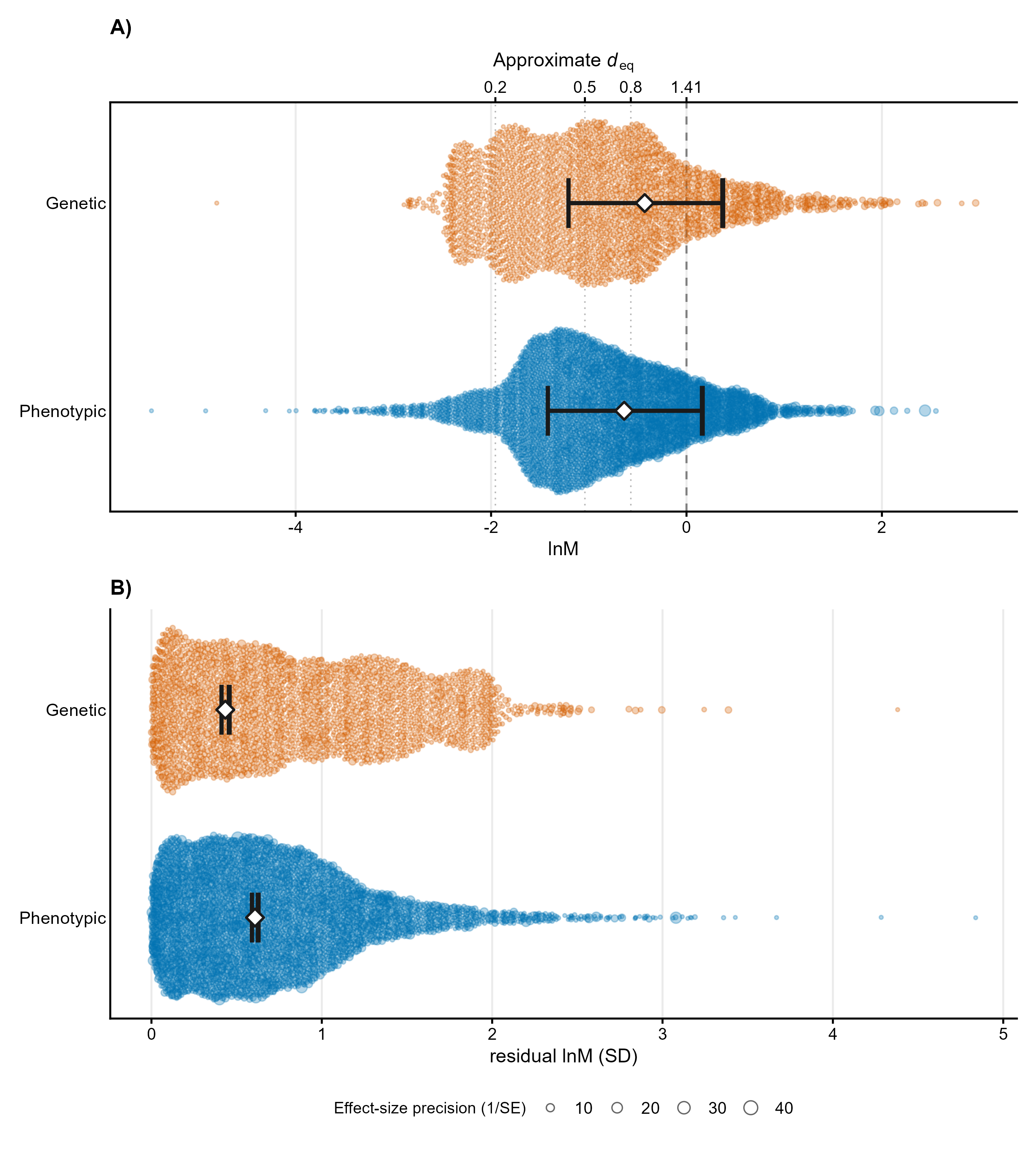
## Orchard-like model figure
The orchard-style figure is read from `Rdata/figures/publication/orchard/`. The complete editable code used to build this plot is shown below.
```{r figure, fig.width=8, fig.height=9}
knitr::include_graphics(
  here::here("Rdata", "figures", "publication", "orchard", "m07_orchard_combined.png")
)
```
### Editable plotting code
The figure above is actually built by `Scripts/17_plot_orchard_from_epred_cache.R`, which reads the credible intervals for each genphen level from `Rdata/summaries/emmeans_contrasts_cache.rds` (`emmeans::emmeans(fit, ~ genphen, epred = TRUE, re_formula = NA)`, i.e. quantiles of the joint posterior of `Intercept + coefficient`). The self-contained variant below is kept for portability; its `get_level_estimates()` uses the same joint-posterior-draws approach rather than the separately computed `Q2.5`/`Q97.5` of the intercept and the coefficient.
```{r build-orchard-m07, eval=FALSE}
library(here)
library(tidyverse)
library(brms)
library(tidybayes)
library(ggbeeswarm)
library(patchwork)

model_id <- "m07"
model_file <- "m07_ls_genphen"
moderator <- "genphen"
moderator_label <- "Phenotypic vs. genetic"
label_map <- c("Genetic" = "Genetic", "Phenotypic" = "Phenotypic")

# Approximate large-sample conversion: |d| = sqrt(2) * exp(lnM).
d_ref <- c(0.2, 0.5, 0.8)
lnm_ref <- log(d_ref / sqrt(2))
d_axis <- ggplot2::sec_axis(
  ~ sqrt(2) * exp(.),
  breaks = c(d_ref, sqrt(2)),
  labels = c("0.2", "0.5", "0.8", "1.41"),
  name = "Approximate |d|"
)

out_dir <- here::here("Rdata", "figures", "publication", "orchard")
out_dir_pdf <- here::here("Figures", "publication", "orchard")
dir.create(out_dir, recursive = TRUE, showWarnings = FALSE)
dir.create(out_dir_pdf, recursive = TRUE, showWarnings = FALSE)

dat_es <- readRDS(here::here("Rdata", "effect_sizes", "proceed_lnm_safe.rds"))
fit <- readRDS(here::here("Rdata", "models", paste0(model_file, ".rds")))

cb_cols <- c("#88CCEE", "#CC6677", "#DDCC77", "#117733", "#332288",
             "#AA4499", "#44AA99", "#999933", "#882255", "#661100",
             "#6699CC", "#888888", "#E69F00", "#56B4E9", "#009E73",
             "#F0E442", "#0072B2", "#D55E00", "#CC79A7", "#999999")

theme_orchard <- function() {
  ggplot2::theme_classic(base_size = 13) +
    ggplot2::theme(
      axis.text.y        = ggplot2::element_text(size = 11),
      axis.title.x       = ggplot2::element_text(size = 12),
      axis.ticks.y       = ggplot2::element_blank(),
      panel.grid.major.x = ggplot2::element_line(colour = "grey92"),
      legend.position    = "bottom",
      legend.title       = ggplot2::element_text(size = 10),
      plot.title         = ggplot2::element_text(size = 13, face = "bold"),
      plot.caption       = ggplot2::element_text(size = 9, colour = "grey50")
    )
}

apply_labels <- function(x, lbl_map) {
  if (is.null(lbl_map)) return(x)
  lbl_map <- lbl_map[!is.na(names(lbl_map))]
  ifelse(x %in% names(lbl_map), lbl_map[x], x)
}

get_level_estimates <- function(fit, moderator) {
  # Credible intervals come from quantiles of the joint posterior draws of
  # (Intercept + coefficient), not from adding the separately-computed
  # Q2.5/Q97.5 of each term — the latter ignores the posterior covariance
  # between the intercept and factor-level coefficients and roughly doubles
  # the interval width.
  draws <- brms::as_draws_df(fit)
  ref_level <- levels(factor(fit$data[[moderator]]))[1]
  pat <- paste0("^b_", moderator)
  coef_cols <- grep(pat, names(draws), value = TRUE)
  cri <- function(d) unname(quantile(d, c(0.025, 0.975)))

  int_draws <- draws[["b_Intercept"]]
  h0 <- cri(int_draws)
  out <- tibble::tibble(
    level = ref_level,
    estimate = mean(int_draws),
    lowerCL = h0[1],
    upperCL = h0[2]
  )
  for (col in coef_cols) {
    lvl <- sub(pat, "", col)
    d <- int_draws + draws[[col]]
    h <- cri(d)
    out <- dplyr::bind_rows(out, tibble::tibble(
      level = lvl,
      estimate = mean(d),
      lowerCL = h[1],
      upperCL = h[2]
    ))
  }
  out
}

get_sig_estimates <- function(fit, moderator, levels_vec = NULL) {
  if (is.null(levels_vec)) {
    levels_vec <- levels(factor(fit$data[[moderator]]))
  }

  nd <- data.frame(x = levels_vec, stringsAsFactors = FALSE)
  names(nd)[1] <- moderator
  nd[["es_id_model"]] <- NA
  nd[["ref_id"]] <- NA
  nd[["sp_ncbi"]] <- NA

  tidybayes::epred_draws(
    fit, newdata = nd, re_formula = NA, dpar = TRUE, ndraws = 1000
  ) |>
    dplyr::group_by(.data[[moderator]]) |>
    dplyr::summarise(
      estimate = mean(sigma),
      lowerCL = quantile(sigma, 0.025),
      upperCL = quantile(sigma, 0.975),
      .groups = "drop"
    ) |>
    dplyr::rename(level = dplyr::all_of(moderator))
}
get_pred_interval <- function(fit, moderator, levels_vec) {
  nd <- data.frame(x = levels_vec, stringsAsFactors = FALSE)
  names(nd)[1] <- moderator
  nd[["es_id_model"]] <- NA
  nd[["ref_id"]] <- NA
  nd[["sp_ncbi"]] <- NA

  pp <- tidybayes::add_predicted_draws(nd, fit, re_formula = NA, ndraws = 1000)
  pp |>
    dplyr::group_by(.data[[moderator]]) |>
    dplyr::summarise(
      lowerPR = quantile(.prediction, 0.025),
      upperPR = quantile(.prediction, 0.975),
      .groups = "drop"
    ) |>
    dplyr::rename(level = dplyr::all_of(moderator))
}

save_plot <- function(p, stem, width = 9, height = 6) {
  ggplot2::ggsave(file.path(out_dir_pdf, paste0(stem, ".pdf")), p,
                  width = width, height = height, device = cairo_pdf)
  ggplot2::ggsave(file.path(out_dir, paste0(stem, ".png")), p,
                  width = width, height = height, dpi = 300, type = "cairo")
}

raw_source <- if (moderator %in% names(dat_es)) dat_es else fit$data
if (!"vi_lnM_safe" %in% names(raw_source) &&
    "es_id_model" %in% names(raw_source) &&
    "es_id_model" %in% names(dat_es)) {
  raw_source <- raw_source |>
    dplyr::left_join(
      dat_es |> dplyr::select(es_id_model, vi_lnM_safe),
      by = "es_id_model"
    )
}

raw <- raw_source[!is.na(raw_source[[moderator]]), ] |>
  dplyr::mutate(
    level = as.character(.data[[moderator]]),
    precision = 1 / sqrt(vi_lnM_safe)
  )

ests <- get_level_estimates(fit, moderator)
sig_ests <- get_sig_estimates(fit, moderator, unique(raw$level))
pi_df <- get_pred_interval(fit, moderator, unique(raw$level))
ests <- dplyr::left_join(ests, pi_df, by = "level")

ests$level <- apply_labels(ests$level, label_map)
sig_ests$level <- apply_labels(sig_ests$level, label_map)
raw$level <- apply_labels(raw$level, label_map)

lev_order <- ests$level[order(ests$estimate)]
ests$level <- factor(ests$level, levels = lev_order)
sig_ests$level <- factor(sig_ests$level, levels = lev_order)
raw$level <- factor(raw$level, levels = lev_order)

n_levels <- nlevels(ests$level)
colors <- cb_cols[seq_len(n_levels)]
names(colors) <- levels(ests$level)

p_loc <- ggplot2::ggplot() +
  ggplot2::geom_vline(xintercept = lnm_ref, linetype = "dotted", colour = "grey72") +
  ggplot2::geom_vline(xintercept = 0, linetype = "dashed", colour = "grey40") +
  ggbeeswarm::geom_quasirandom(
    data = raw,
    ggplot2::aes(x = yi_lnM_safe, y = level,
                 size = precision, colour = level, fill = level),
    alpha = 0.30, shape = 21, groupOnX = FALSE
  ) +
  ggplot2::geom_linerange(
    data = ests,
    ggplot2::aes(y = level, xmin = lowerPR, xmax = upperPR),
    linewidth = 0.4, colour = "grey40"
  ) +
  ggplot2::geom_linerange(
    data = ests,
    ggplot2::aes(y = level, xmin = lowerCL, xmax = upperCL),
    linewidth = 1.5, colour = "grey15"
  ) +
  ggplot2::geom_point(
    data = ests,
    ggplot2::aes(x = estimate, y = level),
    size = 4, shape = 21, fill = "white", colour = "grey10", stroke = 1.2
  ) +
  ggplot2::scale_colour_manual(values = colors, guide = "none") +
  ggplot2::scale_fill_manual(values = colors, guide = "none") +
  ggplot2::scale_size_continuous(name = "Precision (1/SE)", range = c(0.4, 4)) +
  ggplot2::scale_x_continuous(sec.axis = d_axis) +
  ggplot2::labs(
    x = "lnM",
    y = NULL,
    title = "A)"
  ) +
  theme_orchard()

raw_sig <- raw |>
  dplyr::left_join(dplyr::select(ests, level, loc_est = estimate), by = "level") |>
  dplyr::mutate(abs_resid = abs(yi_lnM_safe - loc_est))

p_scl <- ggplot2::ggplot() +
  ggplot2::geom_vline(xintercept = 0, linetype = "dashed", colour = "grey50") +
  ggbeeswarm::geom_quasirandom(
    data = raw_sig,
    ggplot2::aes(x = abs_resid, y = level,
                 size = precision, colour = level, fill = level),
    alpha = 0.30, shape = 21, groupOnX = FALSE
  ) +
  ggplot2::geom_linerange(
    data = sig_ests,
    ggplot2::aes(y = level, xmin = lowerCL, xmax = upperCL),
    linewidth = 3, colour = "white"
  ) +
  ggplot2::geom_linerange(
    data = sig_ests,
    ggplot2::aes(y = level, xmin = lowerCL, xmax = upperCL),
    linewidth = 1.5, colour = "grey15"
  ) +
  ggplot2::geom_point(
    data = sig_ests,
    ggplot2::aes(x = estimate, y = level),
    size = 4, shape = 21, fill = "white", colour = "grey10", stroke = 1.2
  ) +
  ggplot2::scale_colour_manual(values = colors, guide = "none") +
  ggplot2::scale_fill_manual(values = colors, guide = "none") +
  ggplot2::scale_size_continuous(name = "Precision (1/SE)", range = c(0.4, 4)) +
  ggplot2::labs(
    x = "residual lnM (SD)",
    y = NULL,
    title = "B)",
    caption = "Bubbles: absolute residual lnM, sized by precision. Trunk = predicted residual SD (sigma)."
  ) +
  theme_orchard()

p_comb <- patchwork::wrap_plots(p_loc, p_scl, ncol = 1)

height_single <- max(2.5 + n_levels * 0.55, 5)
save_plot(p_loc, paste0(model_id, "_orchard_location"), width = 9, height = height_single)
save_plot(p_scl, paste0(model_id, "_orchard_scale"), width = 9, height = height_single)
save_plot(p_comb, paste0(model_id, "_orchard_combined"), width = 9, height = max(height_single * 1.9, 10))
p_comb
```